GSP631

Overview

TensorFlow is an open source, powerful, portable machine learning (ML) library developed by Google that can work with very large datasets.

In this lab, you will create and train a computer vision model to recognize different items of clothing using TensorFlow on Google Cloud Compute Engine.

What you'll do:

• Set up the development environment in the IDE
• Design, compile, train and evaluate your model
• Save and load models
• Write your own callbacks to customize behaviour during training
• Complete a series of exercises to guide you through experimenting with the different layers of the network

Introduction to TensorFlow

TensorFlow provides a computational framework for building ML models. TensorFlow provides a variety of different toolkits that allow you to construct models at your preferred level of abstraction. In this lab you'll use tf.keras, a high-level API to build and train a neural network for classifying images in TensorFlow.

Neural networks

A neural network is a model inspired from the brain. It is composed of layers, at least one of which is hidden, that consists of simple connected units or neurons followed by nonlinearities.

A node in a neural network typically takes multiple input values and generates one output value. The neuron applies an activation function (nonlinear transformation) to a weighted sum of input values to calculate the output value.

For more information about neural networks, see Neural Networks: Structure.

Setup and requirements

Qwiklabs setup

Before you click the Start Lab button

Read these instructions. Labs are timed and you cannot pause them. The timer, which starts when you click Start Lab, shows how long Google Cloud resources will be made available to you.

This hands-on lab lets you do the lab activities yourself in a real cloud environment, not in a simulation or demo environment. It does so by giving you new, temporary credentials that you use to sign in and access Google Cloud for the duration of the lab.

To complete this lab, you need:

• Access to a standard internet browser (Chrome browser recommended).

Note: Use an Incognito or private browser window to run this lab. This prevents any conflicts between your personal account and the Student account, which may cause extra charges incurred to your personal account.

• Time to complete the lab---remember, once you start, you cannot pause a lab.

Note: If you already have your own personal Google Cloud account or project, do not use it for this lab to avoid extra charges to your account.

Task 1. Access Cloud Code

In this lab, you will be using Cloud Code for creating and running python scripts.

Cloud Code is a set of IDE plugins for popular IDEs that make it easier to create, deploy and integrate applications with Google Cloud.

A Cloud Code development environment has already been set up to easily create and run python scripts.

1. Copy the IDE URL from the lab panel

2. Paste it into a new browser window:

Note: The lab environment is based on a development environment. In this environment, you can run and test the python/tensorflow script from the IDE.

Check for required packages in the IDE environment

1. Open a terminal in the IDE.

Go to Application Menu -> Terminal -> New Terminal

2. Check if your Python environment is already configured. Copy and paste the following command in the terminal.

python --version Incase you get a browser popup while performing the paste command in the IDE terminal, click `Allow` on the popup to enable copy/paste in the IDE.

Example output:

xx:xx:xx ide-dev@cloudlearningservices ~ → python --version Python 3.8.1

3. Check if TensorFlow package is present. Run the following command in the terminal.

python -c "import tensorflow;print(tensorflow.__version__)"

Example output:

xx:xx:xx ide-dev@cloudlearningservices ~ → python -c "import tensorflow;print(tensorflow.__version__)" 2.8.0

The output shows that Python 3.8.1 is already installed, and TensorFlow 2.8.0 is present in your IDE environment.

Install additional packages

To upgrade the pip3, run the following command in the terminal.

pip3 install --upgrade pip

Install google-cloud-logging

You will use google-cloud-logging to write log entries and to manage your Cloud Logging configuration.

To install the google-cloud-logging package, run the following command in the terminal.

/usr/bin/python3 -m pip install -U google-cloud-logging --user

Install pylint

Pylint is a tool that checks for errors in Python code, highlights syntactical and stylistic problems in your Python source code.

To install the pylint package, run the following command in the terminal.

/usr/bin/python3 -m pip install -U pylint --user

Upgrade tensorflow version

To upgrade the tensorflow, run the following command in the terminal.

pip install --upgrade tensorflow

Now, your environment is set up!

Task 2. Start Coding

• Open a new file in the IDE.

Go to Application Menu > File > New File

Task 3. Import necessary packages

1. Import and configure logging and google-cloud-logging for cloud logging.

Add the following code to the file.

# Import and configure logging import logging import google.cloud.logging as cloud_logging from google.cloud.logging.handlers import CloudLoggingHandler from google.cloud.logging_v2.handlers import setup_logging cloud_logger = logging.getLogger('cloudLogger') cloud_logger.setLevel(logging.INFO) cloud_logger.addHandler(CloudLoggingHandler(cloud_logging.Client())) cloud_logger.addHandler(logging.StreamHandler())

2. Import tensorflow for training and evaluating the model. Call it tf for ease of use

Add the following code to the file.

# Import TensorFlow import tensorflow as tf

3. Import numpy, to parse through the data for debugging purposes. Call it np for ease of use.

Add the following code to the file.

# Import numpy import numpy as np

4. Import tensorflow_datasets to integrate the dataset. TensorFlow Datasets is a collection of datasets ready to use, with TensorFlow.

To learn more about how to use it, see the guide and list of datasets. # Import tensorflow_datasets import tensorflow_datasets as tfds

Task 4. Loading and preprocessing the dataset

About the dataset

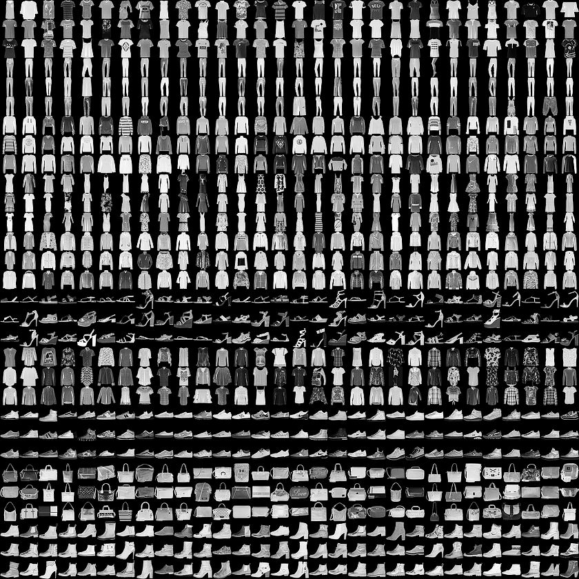
You will train a neural network to classify images of clothing from a dataset called Fashion MNIST.

This dataset contains 70,000 items of clothing belonging to 10 different categories of clothing. The images show individual articles of clothing at low resolution (28 by 28 pixels), as seen here:

In this lab, 60,000 images will be used to train the network and 10,000 images will be used to evaluate how accurately the network learned to classify images.

The Fashion MNIST data is available in tensorflow datasets(tfds).

Loading the dataset

To load the Fashion MNIST data, you will use the tfds.load() function.

1. Add the following code to the end of the file:

# Define, load and configure data (ds_train, ds_test), info = tfds.load('fashion_mnist', split=['train', 'test'], with_info=True, as_supervised=True)

In the above code, you set the split argument to specify which splits of the dataset is to be loaded. You set as_supervised to True to ensure that the loaded tf.data.Dataset will have a 2-tuple structure (input, label).

ds_train and ds_test are of type tf.data.Dataset. ds_train has 60,000 images which will be used for training the model. ds_test has 10,000 images which will be used for evaluating the model.

To read more about tfds.load() and its arguments check the guide.

What do these values look like?

2. Next, add print statements to see the min and max values of training images for item 0.

Add the following code to the end of the file:

# Values before normalization image_batch, labels_batch = next(iter(ds_train)) print("Before normalization ->", np.min(image_batch[0]), np.max(image_batch[0]))

Data Preprocessing

1. Batch size is a term used in machine learning and refers to the number of training examples utilized in one iteration. You will set this to a value of 32.

Specify the batch size by adding the following to model.py:

# Define batch size BATCH_SIZE = 32

2. When training a neural network, for various reasons it's easier if you scale the pixel values to the range between 0 to 1. This process is called 'normalization'. Since the pixel values for FashionMNIST dataset are in the range of [0, 255], you will divide the pixel values by 255.0 to normalize the images.

The code given below uses the map() function of tf.data.Dataset to apply the normalization to images in ds_train and ds_test. Since the pixel values are of type tf.uint8, the tf.cast function is used to convert them to tf.float32 and then divide by 255.0. The dataset is also converted into batches by calling the batch() method with BATCH_SIZE as the argument.

Read more about all the methods available for tf.data.Dataset here.

Add the following code to the end of the file:

# Normalize and batch process the dataset ds_train = ds_train.map(lambda x, y: (tf.cast(x, tf.float32)/255.0, y)).batch(BATCH_SIZE) ds_test = ds_test.map(lambda x, y: (tf.cast(x, tf.float32)/255.0, y)).batch(BATCH_SIZE)

3. Re-print the min and max values of an image in the train dataset:

Add the following code to the end of the file:

# Examine the min and max values of the batch after normalization image_batch, labels_batch = next(iter(ds_train)) print("After normalization ->", np.min(image_batch[0]), np.max(image_batch[0]))

Task 5. Design your model

In this section, you will design your model using TensorFlow.

Add the following code to the file:

# Define the model model = tf.keras.models.Sequential([tf.keras.layers.Flatten(), tf.keras.layers.Dense(64, activation=tf.nn.relu), tf.keras.layers.Dense(10, activation=tf.nn.softmax)])

Look at the different types of layers and the parameters used in the model architecture:

• Sequential: This defines a SEQUENCE of layers in the neural network.

• Flatten: Our images are of shape (28, 28), i.e, the values are in the form of a square matrix. Flatten takes that square and turns it into a one-dimensional vector.

• Dense: Adds a layer of neurons.

Each layer of neurons needs an activation function to decide if a neuron should be activated or not. There are lots of options, but this lab uses the following ones.

• Relu effectively means if X>0 return X, else return 0. It passes values 0 or greater to the next layer in the network.
• Softmax takes a set of values, and effectively picks the biggest one so you don't have to sort to find the largest value. For example, if the output of the last layer looks like [0.1, 0.1, 0.05, 0.1, 9.5, 0.1, 0.05, 0.05, 0.05], it returns [0,0,0,0,1,0,0,0,0].

Task 6. Compile and train the model

In this section you will first compile your model with an optimizer and loss function. You will then train the model on your training data and labels.

The goal is for the model to figure out the relationship between the training data and its labels. Once training is complete, you want your model to see fresh images of clothing that resembles your training data and make predictions about what class of clothing they belong to.

An optimizer is one of the two arguments required for compiling a tf.keras model. An Optimizer is an algorithm that modifies the attributes of the neural network like weights and learning rate. This helps in reducing the loss and improving accuracy.

Read more about different types of optimizers available in tf.keras, here.

Loss indicates the model's performance by a number. If the model is performing better, loss will be a smaller number. Otherwise loss will be a larger number.

Read more about different types of loss functions available in tf.keras here.

Notice the metrics= parameter. This allows TensorFlow to report on the accuracy of the training after each epoch by checking the predicted results against the known answers(labels). It basically reports back on how effectively the training is progressing.

Click here for more details on the different types of metrics available in `tf.keras`

Model.fit will train the model for a fixed number of epochs.

1. Add the following code to the file:

# Compile the model model.compile(optimizer = tf.keras.optimizers.Adam(), loss = tf.keras.losses.SparseCategoricalCrossentropy(), metrics=[tf.keras.metrics.SparseCategoricalAccuracy()]) model.fit(ds_train, epochs=5)

Now your file should look like this:

# Import and configure logging import logging import google.cloud.logging as cloud_logging from google.cloud.logging.handlers import CloudLoggingHandler from google.cloud.logging_v2.handlers import setup_logging cloud_logger = logging.getLogger('cloudLogger') cloud_logger.setLevel(logging.INFO) cloud_logger.addHandler(CloudLoggingHandler(cloud_logging.Client())) cloud_logger.addHandler(logging.StreamHandler()) # Import TensorFlow import tensorflow as tf # Import tensorflow_datasets import tensorflow_datasets as tfds # Import numpy import numpy as np # Define, load and configure data (ds_train, ds_test), info = tfds.load('fashion_mnist', split=['train', 'test'], with_info=True, as_supervised=True) # Values before normalization image_batch, labels_batch = next(iter(ds_train)) print("Before normalization ->", np.min(image_batch[0]), np.max(image_batch[0])) # Define batch size BATCH_SIZE = 32 # Normalize and batch process the dataset ds_train = ds_train.map(lambda x, y: (tf.cast(x, tf.float32)/255.0, y)).batch(BATCH_SIZE) ds_test = ds_test.map(lambda x, y: (tf.cast(x, tf.float32)/255.0, y)).batch(BATCH_SIZE) # Examine the min and max values of the batch after normalization image_batch, labels_batch = next(iter(ds_train)) print("After normalization ->", np.min(image_batch[0]), np.max(image_batch[0])) # Define the model model = tf.keras.models.Sequential([tf.keras.layers.Flatten(), tf.keras.layers.Dense(64, activation=tf.nn.relu), tf.keras.layers.Dense(10, activation=tf.nn.softmax)]) # Compile the model model.compile(optimizer = tf.keras.optimizers.Adam(), loss = tf.keras.losses.SparseCategoricalCrossentropy(), metrics=[tf.keras.metrics.SparseCategoricalAccuracy()]) model.fit(ds_train, epochs=5)

2. Press Ctrl + s or go toApplication Menu -> File -> Save. In the prompt, type model.py for name and press OK.

Click Check my progress to verify the objective. Create machine learning models

Run the script

Your script is ready! Run it to see what happens. Enter the following command in the terminal:

python model.py

When the script executes, you will see both loss and accuracy reported after each epoch (or pass) of training. Notice that with each epoch (or pass), the accuracy goes up:

Example output (your values may be slightly different, ignore any warning messages):

Before normalization -> 0 227 After normalization -> 0.0 1.0 Epoch 1/5 1875/1875 [==============================] - 12s 6ms/step - loss: 0.5264 - sparse_categorical_accuracy: 0.8175 Epoch 2/5 1875/1875 [==============================] - 6s 3ms/step - loss: 0.3977 - sparse_categorical_accuracy: 0.8580 Epoch 3/5 1875/1875 [==============================] - 5s 3ms/step - loss: 0.3585 - sparse_categorical_accuracy: 0.8701 Epoch 4/5 1875/1875 [==============================] - 5s 2ms/step - loss: 0.3329 - sparse_categorical_accuracy: 0.8784 Epoch 5/5 1875/1875 [==============================] - 5s 2ms/step - loss: 0.3151 - sparse_categorical_accuracy: 0.8846

For # Values before normalization output, you'll notice that the min and max are in the range of [0, 255]. After normalization you can see that all the values are in the range of [0, 1].

As the training progresses, the loss decreases and accuracy increases.

When the model is done training, you will see an accuracy value at the end of the final epoch. It might be close to 0.8864 as above (your accuracy may be different).

This tells you that the neural network is about 89% accurate in classifying the training data. In other words, it figured out a pattern match between the image and the labels that worked 89% of the time. Not great, but not bad considering it was only trained for five epochs on a small neural network.

Task 7. Evaluate model performance on unseen data

But how would the model perform on data it hasn't seen?

The test set can help answer this question. You call model.evaluate, pass in the two sets, and it reports back the loss for each.

Evaluate the test set:

1. Add the following code to model.py evaluate model performance. You will also log evaluation results to our log file.

cloud_logger.info(model.evaluate(ds_test))

2. Press Ctrl+s or go toApplication Menu -> File -> Save, to save the changes.

3. Run the script. Enter the following command in the terminal:

python model.py

If you scroll to the bottom of your output, you can see the result of evaluation in the last line.

Before normalization -> 0 227 After normalization -> 0.0 1.0 Epoch 1/5 1875/1875 [==============================] - 12s 6ms/step - loss: 0.5264 - sparse_categorical_accuracy: 0.8175 Epoch 2/5 1875/1875 [==============================] - 6s 3ms/step - loss: 0.3977 - sparse_categorical_accuracy: 0.8580 Epoch 3/5 1875/1875 [==============================] - 5s 3ms/step - loss: 0.3585 - sparse_categorical_accuracy: 0.8701 Epoch 4/5 1875/1875 [==============================] - 5s 2ms/step - loss: 0.3329 - sparse_categorical_accuracy: 0.8784 Epoch 5/5 1875/1875 [==============================] - 5s 2ms/step - loss: 0.3151 - sparse_categorical_accuracy: 0.8846 313/313 [==============================] - 1s 4ms/step - loss: 0.3653 - sparse_categorical_accuracy: 0.8708 INFO:cloudLogger:[0.36530008912086487, 0.8708000183105469]

The model reports an accuracy of .8708 on the test set(ds_test), meaning it was about 87% accurate. (Your values may be slightly different).

As expected, the model is not as accurate on the unknown data as it was with the data it was trained on!

As you dive deeper into TensorFlow, you'll learn about ways to improve this.

Click Check my progress to verify the objective. Use the model

Task 8. Saving and loading the model

Model progress can be saved during and after training. This means a model can resume where it left off and avoid long training times. Saving also means you can share your model and others can recreate your work. For this first exercise, you will add necessary code to save and load your model.

An entire model can be saved in two different file formats (SavedModel and HDF5). The TensorFlow SavedModel format is the default file format in TF2.x. However, models can be saved in HDF5 format. You will learn more on saving models in the two file formats.

1. Add the following code to the bottom of model.py to save the model in each format(SavedModel and HDF5).

# Save the entire model as a SavedModel. model.save('saved_model') # Reload a fresh Keras model from the saved model new_model = tf.keras.models.load_model('saved_model') # Summary of loaded SavedModel new_model.summary() # Save the entire model to a HDF5 file. model.save('my_model.h5') # Recreate the exact same model, including its weights and the optimizer new_model_h5 = tf.keras.models.load_model('my_model.h5') # Summary of loaded h5 model new_model_h5.summary()

The above code shows how you can save the model in two different formats and load the saved model back. You can choose any format according to your use case. You can read more about this functionality in the TensorFlow Documentation for "Save and load models".

2. Press Ctrl+s or go toApplication Menu -> File -> Save, to save the changes.

3. Run the script. Enter the following command in the terminal:

python model.py

At the end of the output you will see two sets of model summaries. The first one shows the summary after the model is saved in the SavedModel format. The second one shows the summary after the model is saved in the h5 format.

You can see that both model summaries are identical since we are effectively saving the same model in two different formats.

Model: "sequential" _________________________________________________________________ Layer (type) Output Shape Param # ================================================================= flatten (Flatten) (None, 784) 0 dense (Dense) (None, 64) 50240 dense_1 (Dense) (None, 10) 650 ================================================================= Total params: 50,890 Trainable params: 50,890 Non-trainable params: 0 _________________________________________________________________ Model: "sequential" _________________________________________________________________ Layer (type) Output Shape Param # ================================================================= flatten (Flatten) (None, 784) 0 dense (Dense) (None, 64) 50240 dense_1 (Dense) (None, 10) 650 ================================================================= Total params: 50,890 Trainable params: 50,890 Non-trainable params: 0 _________________________________________________________________

Click Check my progress to verify the objective. Save and Load Models

Task 9. Explore callbacks

Earlier when you trained the model, you would have noticed that, as the training progressed, the model's loss decreased and its accuracy increased. Once you have achieved the desired training accuracy and loss, you may still have to wait for a bit of time for the training to complete.

You might have thought, "Wouldn't it be nice if I could stop training when the model reached a desired value of accuracy?"

For example, if 95% accuracy is good enough, and the model managed to achieve that after 3 epochs of training, why sit around waiting for many more epochs to complete?

Answer: Callbacks!

A callback is a powerful tool to customize the behavior of a Keras model during training, evaluation, or inference. You can define a callback to stop training as soon as your model reaches a desired accuracy on the training set.

Try the following code to see what happens when you set a callback to stop training when accuracy reaches 84%:

1. Open a new file in IDE.

Go to Application Menu -> File -> New File

2. Press Ctrl + s or go toApplication Menu -> File -> Save. In the prompt, type callback_model.py for name and press OK.

3. Paste the following code into callback_model.py:

# Import and configure logging import logging import google.cloud.logging as cloud_logging from google.cloud.logging.handlers import CloudLoggingHandler from google.cloud.logging_v2.handlers import setup_logging exp_logger = logging.getLogger('expLogger') exp_logger.setLevel(logging.INFO) exp_logger.addHandler(CloudLoggingHandler(cloud_logging.Client(), name="callback")) # Import tensorflow_datasets import tensorflow_datasets as tfds # Import numpy import numpy as np # Import TensorFlow import tensorflow as tf # Define Callback class myCallback(tf.keras.callbacks.Callback): def on_epoch_end(self, epoch, logs={}): if(logs.get('sparse_categorical_accuracy')>0.84): exp_logger.info("\nReached 84% accuracy so cancelling training!") self.model.stop_training = True callbacks = myCallback() # Define, load and configure data (ds_train, ds_test), info = tfds.load('fashion_mnist', split=['train', 'test'], with_info=True, as_supervised=True) # Define batch size BATCH_SIZE = 32 # Normalizing and batch processing of data ds_train = ds_train.map(lambda x, y: (tf.cast(x, tf.float32)/255.0, y)).batch(BATCH_SIZE) ds_test = ds_test.map(lambda x, y: (tf.cast(x, tf.float32)/255.0, y)).batch(BATCH_SIZE) # Define the model model = tf.keras.models.Sequential([tf.keras.layers.Flatten(), tf.keras.layers.Dense(64, activation=tf.nn.relu), tf.keras.layers.Dense(10, activation=tf.nn.softmax)]) # Compile data model.compile(optimizer = tf.keras.optimizers.Adam(), loss = tf.keras.losses.SparseCategoricalCrossentropy(), metrics=[tf.keras.metrics.SparseCategoricalAccuracy()]) model.fit(ds_train, epochs=5, callbacks=[callbacks])

4. Press Ctrl + s or go toApplication Menu -> File -> Save, to save the changes.

5. Run the script. Enter the following command in the terminal:

python callback_model.py

See that the training was canceled after a few epochs.

Click Check my progress to verify the objective. Explore Callbacks

Explore

In this section you will experiment with the different layers of the network.

Exercise 1

In this Exercise you will explore the layers in your model. What happens when you change the number of neurons?

1. Open a new file in IDE.

Go to Application Menu -> File -> New File

2. Press Ctrl + s or go toApplication Menu -> File -> Save. In the prompt, type updated_model.py for name and press OK.

3. Paste the following code into updated_model.py:

# Import and configure logging import logging import google.cloud.logging as cloud_logging from google.cloud.logging.handlers import CloudLoggingHandler from google.cloud.logging_v2.handlers import setup_logging up_logger = logging.getLogger('upLogger') up_logger.setLevel(logging.INFO) up_logger.addHandler(CloudLoggingHandler(cloud_logging.Client(), name="updated")) # Import tensorflow_datasets import tensorflow_datasets as tfds # Import numpy import numpy as np # Import TensorFlow import tensorflow as tf # Define, load and configure data (ds_train, ds_test), info = tfds.load('fashion_mnist', split=['train', 'test'], with_info=True, as_supervised=True) # Define batch size BATCH_SIZE = 32 # Normalizing and batch processing of data ds_train = ds_train.map(lambda x, y: (tf.cast(x, tf.float32)/255.0, y)).batch(BATCH_SIZE) ds_test = ds_test.map(lambda x, y: (tf.cast(x, tf.float32)/255.0, y)).batch(BATCH_SIZE) # Define the model model = tf.keras.models.Sequential([tf.keras.layers.Flatten(), tf.keras.layers.Dense(64, activation=tf.nn.relu), tf.keras.layers.Dense(10, activation=tf.nn.softmax)]) # Compile data model.compile(optimizer = tf.keras.optimizers.Adam(), loss = tf.keras.losses.SparseCategoricalCrossentropy(), metrics=[tf.keras.metrics.SparseCategoricalAccuracy()]) model.fit(ds_train, epochs=5) # Logs model summary model.summary(print_fn=up_logger.info)

4. Experiment with different values for the dense layer.

Go to # Define the model section, change 64 to 128 neurons:

# Define the model model = tf.keras.models.Sequential([tf.keras.layers.Flatten(), tf.keras.layers.Dense(128, activation=tf.nn.relu), tf.keras.layers.Dense(10, activation=tf.nn.softmax)])

5. Press Ctrl + s or go toApplication Menu -> File -> Save, to save the changes.

6. Run the script. Enter the following command in the terminal:

python updated_model.py

What different results do you get for loss, training time, etc.? Why do you think that's the case?

When you increase to 128 neurons, you have to do more calculations. This slows down the training process. In this case, the increase had a positive impact because the model is more accurate. But, it's not always a case of 'more is better'. You can hit the law of diminishing returns very quickly.

Click Check my progress to verify the objective. Exercise 1

Exercise 2

Consider the effects of additional layers in the network. What will happen if you add another layer between the two dense layers?

1. In updated_model.py, add a layer in the # Define the model section.

Replace your model definition with the following:

# Define the model model = tf.keras.models.Sequential([tf.keras.layers.Flatten(), tf.keras.layers.Dense(64, activation=tf.nn.relu), tf.keras.layers.Dense(64, activation=tf.nn.relu), tf.keras.layers.Dense(10, activation=tf.nn.softmax)])

2. Press Ctrl + s or go toApplication Menu -> File -> Save, to save the changes.

3. Run the script. Enter the following command in the terminal:

python updated_model.py

Answer: No significant impact -- because this is relatively simple data. For far more complex data, extra layers are often necessary.

Click Check my progress to verify the objective. Exercise 2

Exercise 3

Before you trained your model, you normalized the pixel values to the range of [0, 1]. What would be the impact of removing normalization so that the values are in the range of [0, 255], like they were originally in the dataset?

1. Give it a try -- in the # Normalize the data section, remove the map function applied to both the training and test datasets.

# Define batch size BATCH_SIZE = 32 # Normalizing and batch processing of data ds_train = ds_train.batch(BATCH_SIZE) ds_test = ds_test.batch(BATCH_SIZE) # Define the model model = tf.keras.models.Sequential([tf.keras.layers.Flatten(), tf.keras.layers.Dense(64, activation=tf.nn.relu), tf.keras.layers.Dense(10, activation=tf.nn.softmax)])

2. Add this code at the end of updated_model.py to print the max value of the first image in batch 0. Without normalization, the max value will be in the range of [0, 255].

# Print out max value to see the changes image_batch, labels_batch = next(iter(ds_train)) t_image_batch, t_labels_batch = next(iter(ds_test)) up_logger.info("training images max " + str(np.max(image_batch[0]))) up_logger.info("test images max " + str(np.max(t_image_batch[0])))

3. Your final updated_model.py will look like this

# Import and configure logging import logging import google.cloud.logging as cloud_logging from google.cloud.logging.handlers import CloudLoggingHandler from google.cloud.logging_v2.handlers import setup_logging up_logger = logging.getLogger('upLogger') up_logger.setLevel(logging.INFO) up_logger.addHandler(CloudLoggingHandler(cloud_logging.Client(), name="updated")) # Import tensorflow_datasets import tensorflow_datasets as tfds # Import numpy import numpy as np # Import TensorFlow import tensorflow as tf # Define, load and configure data (ds_train, ds_test), info = tfds.load('fashion_mnist', split=['train', 'test'], with_info=True, as_supervised=True) # Define batch size BATCH_SIZE = 32 # Normalizing and batch processing of data ds_train = ds_train.batch(BATCH_SIZE) ds_test = ds_test.batch(BATCH_SIZE) # Define the model model = tf.keras.models.Sequential([tf.keras.layers.Flatten(), tf.keras.layers.Dense(64, activation=tf.nn.relu), tf.keras.layers.Dense(10, activation=tf.nn.softmax)]) # Compile data model.compile(optimizer = tf.keras.optimizers.Adam(), loss = tf.keras.losses.SparseCategoricalCrossentropy(), metrics=[tf.keras.metrics.SparseCategoricalAccuracy()]) model.fit(ds_train, epochs=5) # Logs model summary model.summary(print_fn=up_logger.info) # Print out max value to see the changes image_batch, labels_batch = next(iter(ds_train)) t_image_batch, t_labels_batch = next(iter(ds_test)) up_logger.info("training images max " + str(np.max(image_batch[0]))) up_logger.info("test images max " + str(np.max(t_image_batch[0])))

4. Press Ctrl + s or go toApplication Menu -> File -> Save, to save the changes.

5. Run the script. Enter the following command in the terminal:

python updated_model.py

Expected output for # Print out max value to see the changes

INFO:upLogger:training images max 255 INFO:upLogger:test images max 255

After completing the epochs you can see the difference in accuracy without normalization.

Why do you think the accuracy changes?

There's a great answer here on Stack Overflow.

Click Check my progress to verify the objective. Exercise 3

Exercise 4

What happens if you remove the Flatten() layer, and why?

Go ahead, try it:

1. In the # Define the model section, remove "tf.keras.layers.Flatten()":

# Define the model model = tf.keras.models.Sequential([tf.keras.layers.Dense(64, activation=tf.nn.relu), tf.keras.layers.Dense(10, activation=tf.nn.softmax)])

2. Save and run updated_model.py.

You get an error about the shape of the data. This is expected.

The details of the error may seem vague right now, but it reinforces the rule of thumb that the first layer in your network should be the same shape as your data. Right now, the input images are of shape 28x28, and 28 layers of 28 neurons would be infeasible. So, it makes more sense to flatten that 28,28 into a 784x1.

Instead of writing all the code to handle that yourselves, you can add the Flatten() layer at the beginning. When the arrays are loaded into the model later, they'll automatically be flattened for you.

Exercise 5

Notice the final (output) layer. Why are there 10 neurons in the final layer? What happens if you have a different number than 10?

Find out by training the network with 5.

1. Replace the # Define the model section with the following to undo the change you made in the previous section:

# Define the model model = tf.keras.models.Sequential([tf.keras.layers.Flatten(), tf.keras.layers.Dense(64, activation=tf.nn.relu), tf.keras.layers.Dense(10, activation=tf.nn.softmax)])

2. Change the number of neurons in the last layer from 10 to 5:

# Define the model model = tf.keras.models.Sequential([tf.keras.layers.Flatten(), tf.keras.layers.Dense(64, activation=tf.nn.relu), tf.keras.layers.Dense(5, activation=tf.nn.softmax)])

3. Save and run updated_model.py.

What happens: You get an error as soon as it finds an unexpected value.

Another rule of thumb -- the number of neurons in the last layer should match the number of classes you are classifying for. In this case, it's the digits 0-9, so there are 10 of them, and hence you should have 10 neurons in your final layer.

Congratulations!

This concludes the self-paced lab, Introduction to Computer Vision with TensorFlow. After you created, trained, and tested your ML model, you experimented by changing the model , saving the model in different formats and creating a callback.

Next steps / learn more

• See all there is to know at Machine Learning Crash Course.
• Have fun trying out Try it! to get a feel for what you can do with computer vision.
• Check out machine learning as part of the AI Platform, see AI Platform documentation.
• Fun stuff with AI! See Experiments with Google.
• Learn more about TensorFlow.

Google Cloud training and certification

...helps you make the most of Google Cloud technologies. Our classes include technical skills and best practices to help you get up to speed quickly and continue your learning journey. We offer fundamental to advanced level training, with on-demand, live, and virtual options to suit your busy schedule. Certifications help you validate and prove your skill and expertise in Google Cloud technologies.

Manual Last Updated October 03, 2023

Lab Last Tested October 05, 2023

Copyright 2024 Google LLC All rights reserved. Google and the Google logo are trademarks of Google LLC. All other company and product names may be trademarks of the respective companies with which they are associated.