Checkpoints
Enable Visual Inspection AI API
/ 35
Create a Dataset
/ 35
Import training images into the dataset
/ 30
Create a Cosmetic Anomaly Detection Model using Visual Inspection AI
- GSP897
- Overview
- Objectives
- Setup and requirements
- Task 1. Create a dataset
- Task 2. Import training images into the dataset
- Task 3. Provide annotation for defect instances in training images
- Overview 1. Evaluating a trained Cosmetic Inspection model
- Overview 2. Creating a trained Cosmetic Inspection solution artifact
- Overview 3. Performing batch predictions using a Cosmetic Inspection solution artifact
- Congratulations
GSP897

Overview
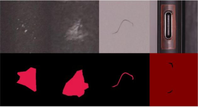
Visual Inspection AI Cosmetic Inspection inspects products to detect and recognize defects such as dents, scratches, cracks, deformations, foreign materials, etc. on any kind of surface such as those shown in the following image.
In this lab, you will upload a collection of training images and then annotate these training images with a set of sample defect instances to facilitate Cosmetic Inspection solution training. You will then use the UI to prepare a Visual Inspection AI Cosmetic Inspection model for training.
Model training can take a a long time so this lab is paired with Deploy and Test a Visual Inspection AI Cosmetic Anomaly Detection Solution where you deploy the Visual Inspection solution artifact created in this lab and then use that artifact to generate inferences about sample images.
Objectives
In this lab, you will learn how to complete the following tasks:
- Enable the Visual Inspection AI API.
- Create a Visual Inspection AI Cosmetic Inspection dataset.
- Import training images to train a Visual Inspection AI Cosmetic Inspection model.
- Provide annotations for defect instances in the training images.
- Review the process involved in evaluation of a trained Cosmetic Inspection model.
- Review the process of creating a trained Cosmetic Inspection solution artifact.
- Review the process of performing batch prediction using an Cosmetic Inspection solution artifact.
Setup and requirements
Before you click the Start Lab button
Read these instructions. Labs are timed and you cannot pause them. The timer, which starts when you click Start Lab, shows how long Google Cloud resources will be made available to you.
This hands-on lab lets you do the lab activities yourself in a real cloud environment, not in a simulation or demo environment. It does so by giving you new, temporary credentials that you use to sign in and access Google Cloud for the duration of the lab.
To complete this lab, you need:
- Access to a standard internet browser (Chrome browser recommended).
- Time to complete the lab---remember, once you start, you cannot pause a lab.
How to start your lab and sign in to the Google Cloud console
-
Click the Start Lab button. If you need to pay for the lab, a pop-up opens for you to select your payment method. On the left is the Lab Details panel with the following:
- The Open Google Cloud console button
- Time remaining
- The temporary credentials that you must use for this lab
- Other information, if needed, to step through this lab
-
Click Open Google Cloud console (or right-click and select Open Link in Incognito Window if you are running the Chrome browser).
The lab spins up resources, and then opens another tab that shows the Sign in page.
Tip: Arrange the tabs in separate windows, side-by-side.
Note: If you see the Choose an account dialog, click Use Another Account. -
If necessary, copy the Username below and paste it into the Sign in dialog.
{{{user_0.username | "Username"}}} You can also find the Username in the Lab Details panel.
-
Click Next.
-
Copy the Password below and paste it into the Welcome dialog.
{{{user_0.password | "Password"}}} You can also find the Password in the Lab Details panel.
-
Click Next.
Important: You must use the credentials the lab provides you. Do not use your Google Cloud account credentials. Note: Using your own Google Cloud account for this lab may incur extra charges. -
Click through the subsequent pages:
- Accept the terms and conditions.
- Do not add recovery options or two-factor authentication (because this is a temporary account).
- Do not sign up for free trials.
After a few moments, the Google Cloud console opens in this tab.
Activate Cloud Shell
Cloud Shell is a virtual machine that is loaded with development tools. It offers a persistent 5GB home directory and runs on the Google Cloud. Cloud Shell provides command-line access to your Google Cloud resources.
- Click Activate Cloud Shell
at the top of the Google Cloud console.
When you are connected, you are already authenticated, and the project is set to your Project_ID,
gcloud is the command-line tool for Google Cloud. It comes pre-installed on Cloud Shell and supports tab-completion.
- (Optional) You can list the active account name with this command:
- Click Authorize.
Output:
- (Optional) You can list the project ID with this command:
Output:
gcloud, in Google Cloud, refer to the gcloud CLI overview guide.
Task 1. Create a dataset
In this task, you will enable the Visual Inspection AI API and create a new Visual Inspection AI Cosmetic Inspection training dataset.
-
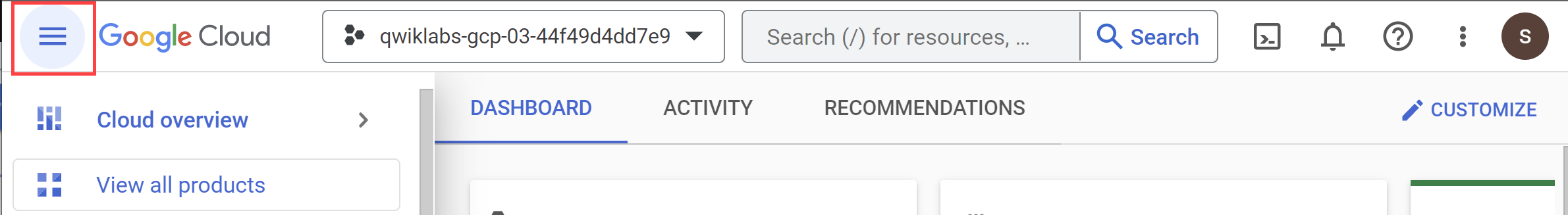
In the Navigation Menu, click Visual Inspection AI to open the Visual Inspection console.
-
Click the Enable Visual Inspection AI API button.
Click Check my progress to verify the objective.
-
Click Create a Dataset.
-
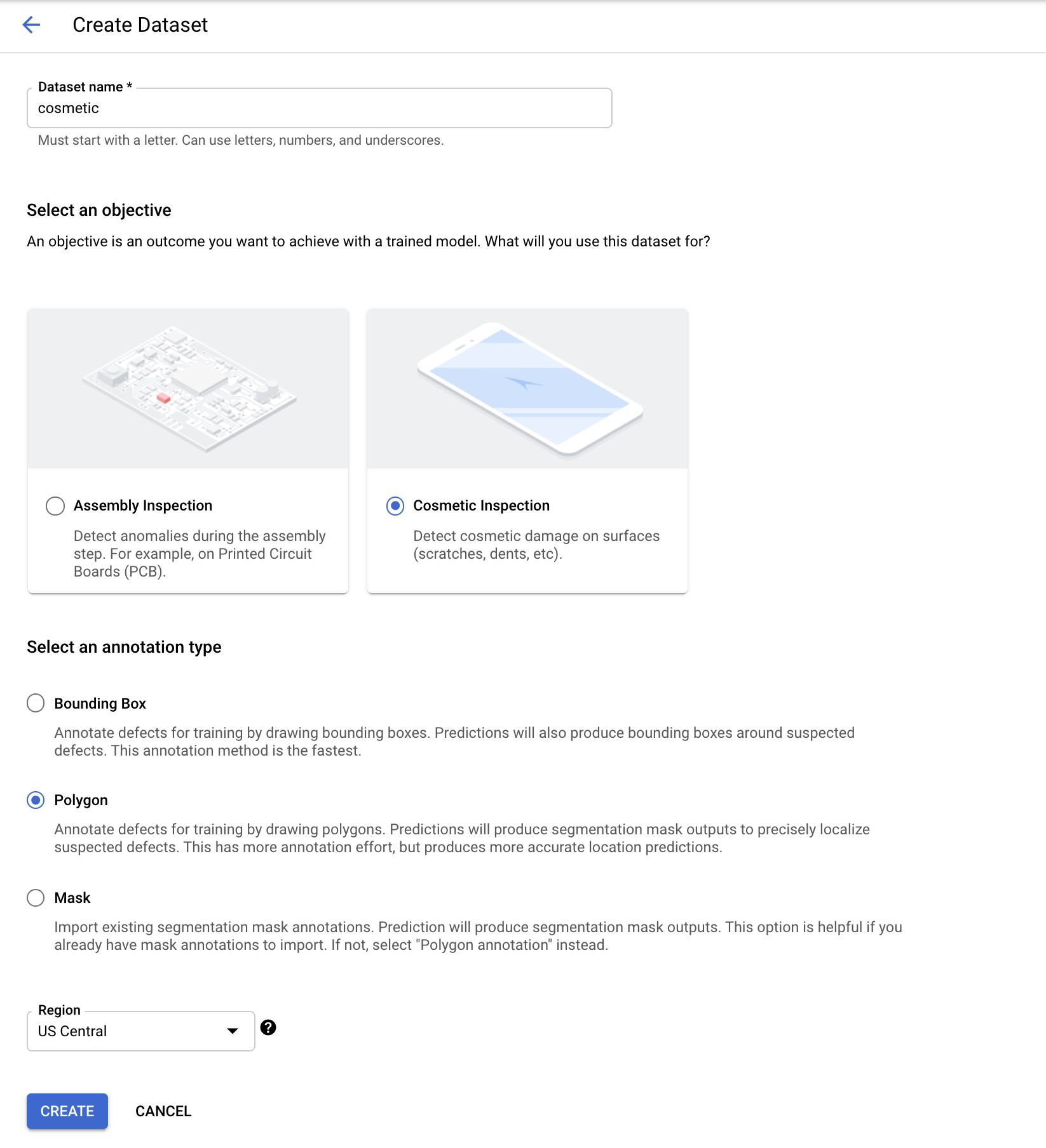
In the Create Dataset page:
- For Dataset name, enter cosmetic
- For Objective select Cosmetic Inspection.
- For Annotation type select Polygon.
- For Region, select US Central1.
-
Click Create.
Dataset creation will take a minute or two to complete.
Click Check my progress to verify the objective.
Task 2. Import training images into the dataset
In this task, you will import the training images into the Dataset. You will use a Google Visual Inspection demo dataset to follow along with the instructions below. This dataset consists of a set of sample product images some of which include sample defects that you will have to locate and identify to prepare the dataset for training. To upload the images you must upload a CSV file that contains a list of Cloud Storage paths to the sample images that are to be included into the Visual Inspection AI Cosmetic Inspection model training.
- In Cloud Shell, run the commands below to copy images to your Cloud Storage bucket:
Copying will take a few minutes.
- Create the CSV import file using the following commands:
-
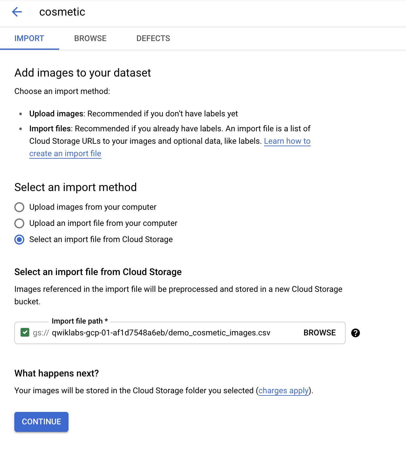
Back in the Visual Inspection AI console, on the Import tab, under Select an import method, select Select an import file from Cloud Storage.
-
In Import File Path, click Browse.
-
Expand the bucket with a name that matches the lab project ID.
-
Select the demo_cosmetic_images.csv import file.
-
Click Select.
-
Click Continue.
A status bar will appear to indicate Import in progress.
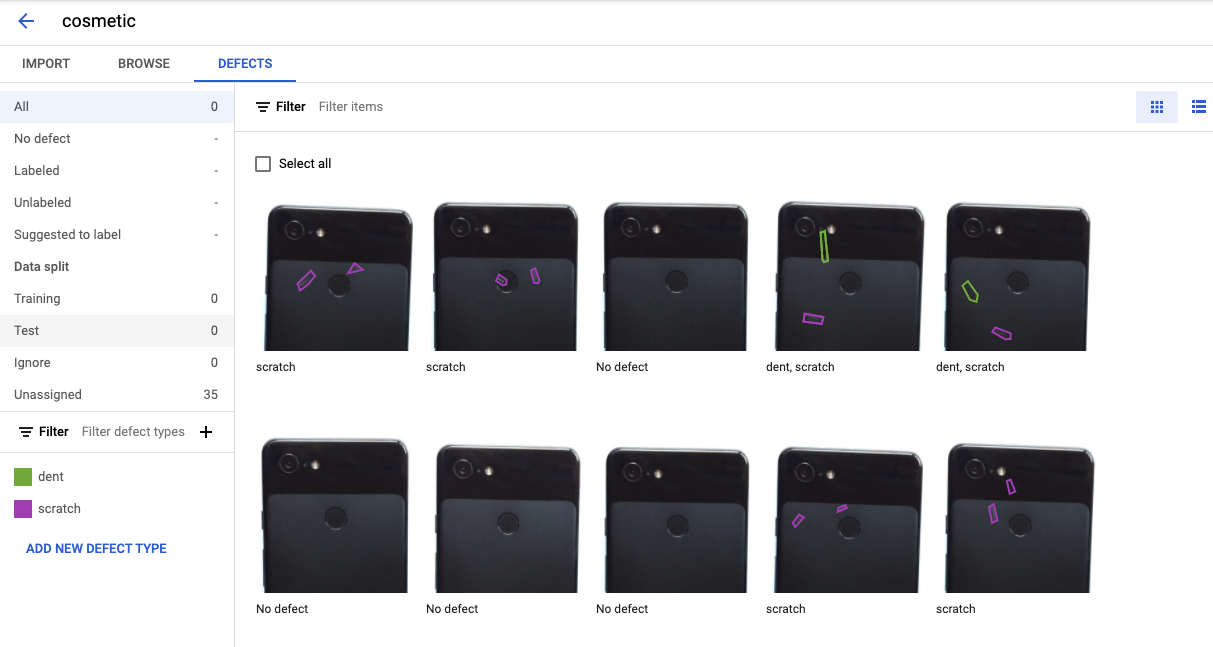
The import will take a few minutes to complete. Once the import is completed, you should see the imported images displayed in the Visual Inspection AI user interface as shown below:
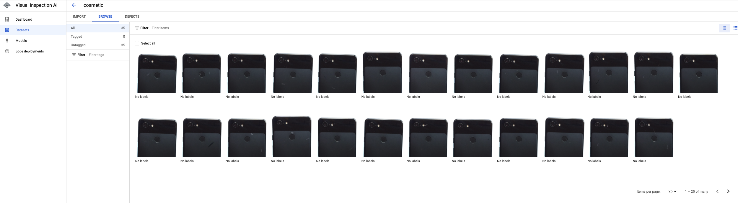
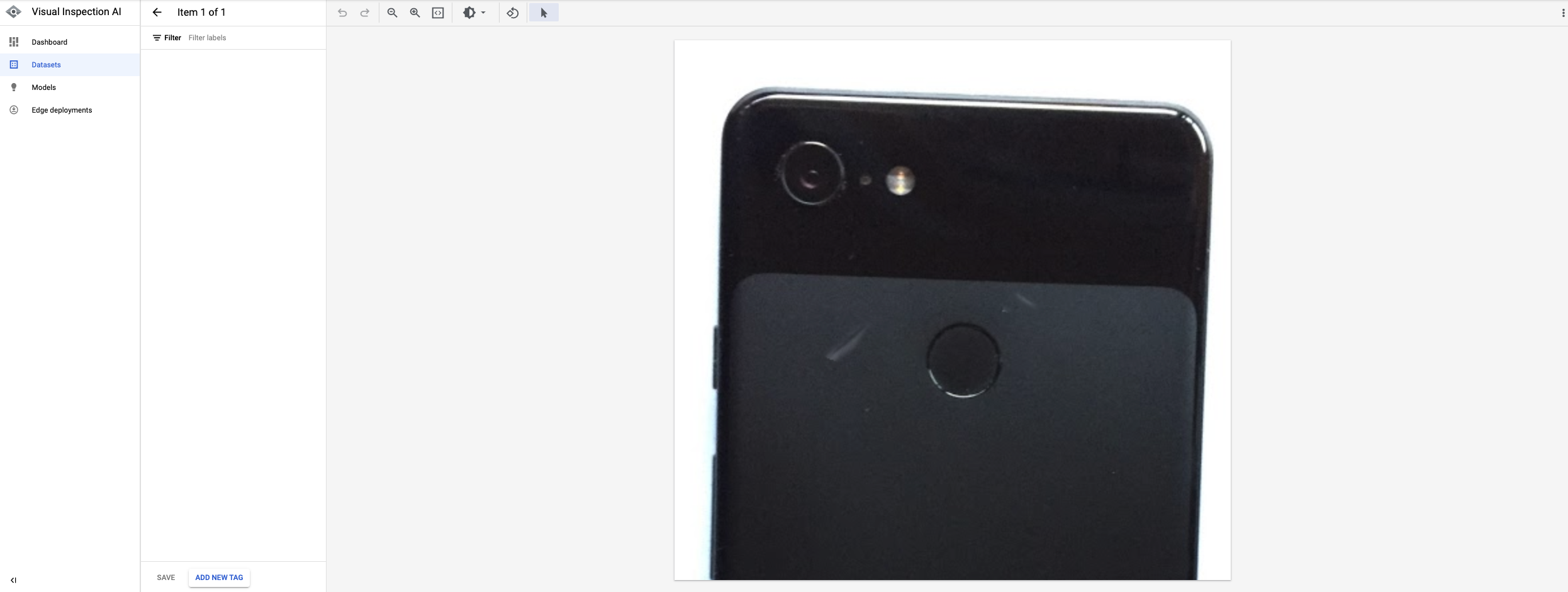
Now that you are able to see the list of imported images, you can browse through them and Click any of the images to have a close-up view as you explore your dataset.
Click Check my progress to verify the objective.
Task 3. Provide annotation for defect instances in training images
In this task, you will annotate sample defect instances using a polygon shape. The Visual Inspection AI Cosmetic Inspection solution learns to detect and localize small and subtle defect instances, such as dents, scratches, and foreign materials visible in the training images by training a dedicated defect instance localization model.
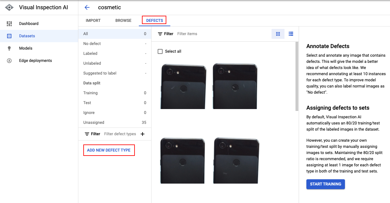
- Click Defects on the Visual Inspection console.
Depending on the Cosmetic Inspection problem, you will need to define defect instance types, which will be subsequently used to associate specific defect instance polygon shapes that you annotate in sample images with specific defect types.
- Click Add New Defect Type.
-
For Defect type, enter dent then select Done and click Create.
-
Click Add New Defect Type
-
For Defect type, enter scratch then select Done and click Create.
After defining the defect types, you can start browsing each individual imported image to provide detailed annotations for each visible defect instance, falling into one of the predefined defect types.
-
Click each image to get the close-up view of the image to annotate your defect instance.
-
Select an image with a defect.
-
Click the Add Simple Polygon icon in the close-up view of the image to start annotating images with defect instances.
-
Locate a concrete defect instance on the image and then provide polygon vertices to annotate the instance.
-
Select a defect type from your previously defined defect type list, either dent or scratch, that matches the defect type you have just annotated.
-
Click Save.
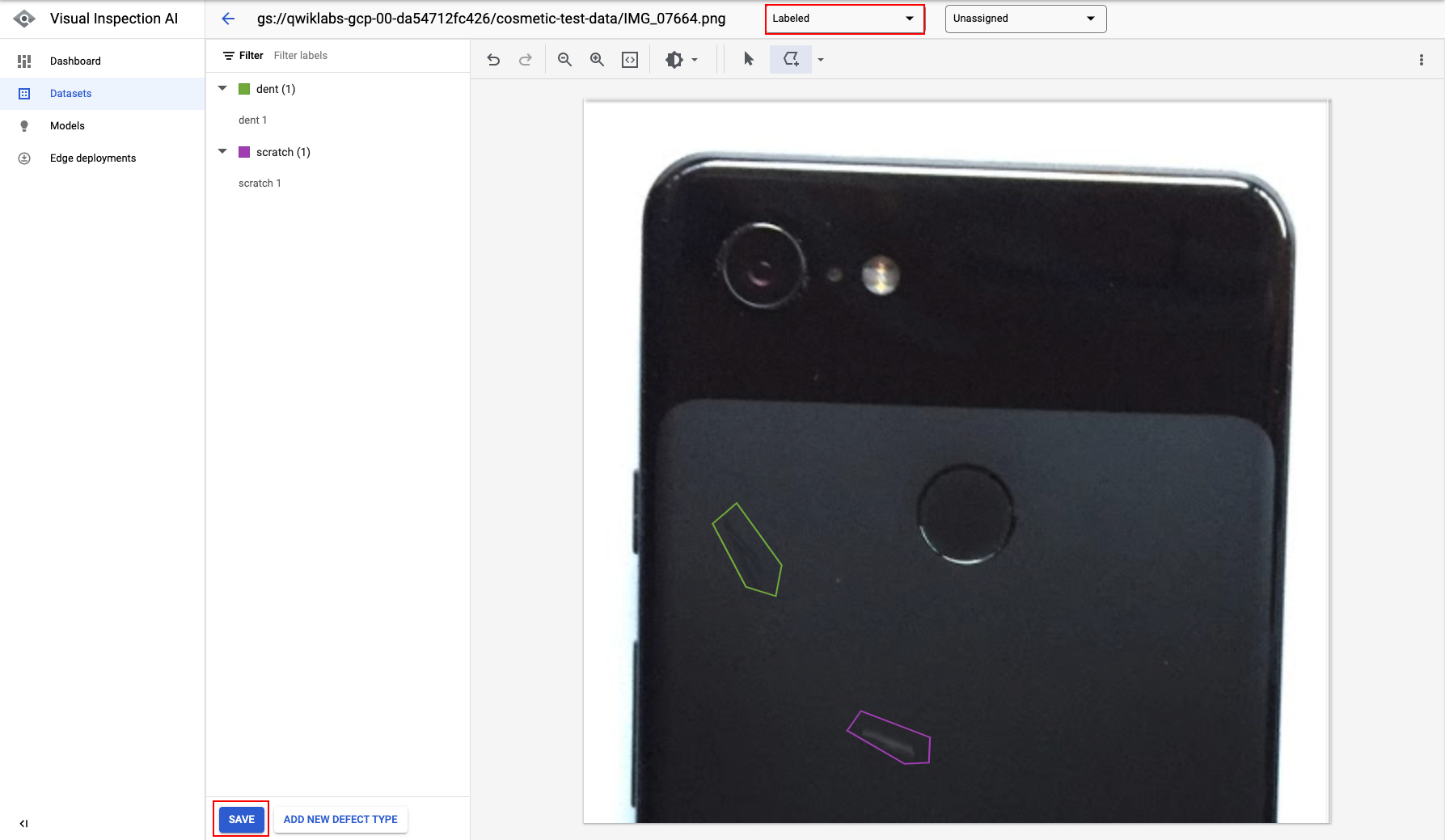
A fully labelled annotation of an image is shown below, where 2 defect instances were identified in the image, one dent and one scratch with their corresponding polygon shaped locations.
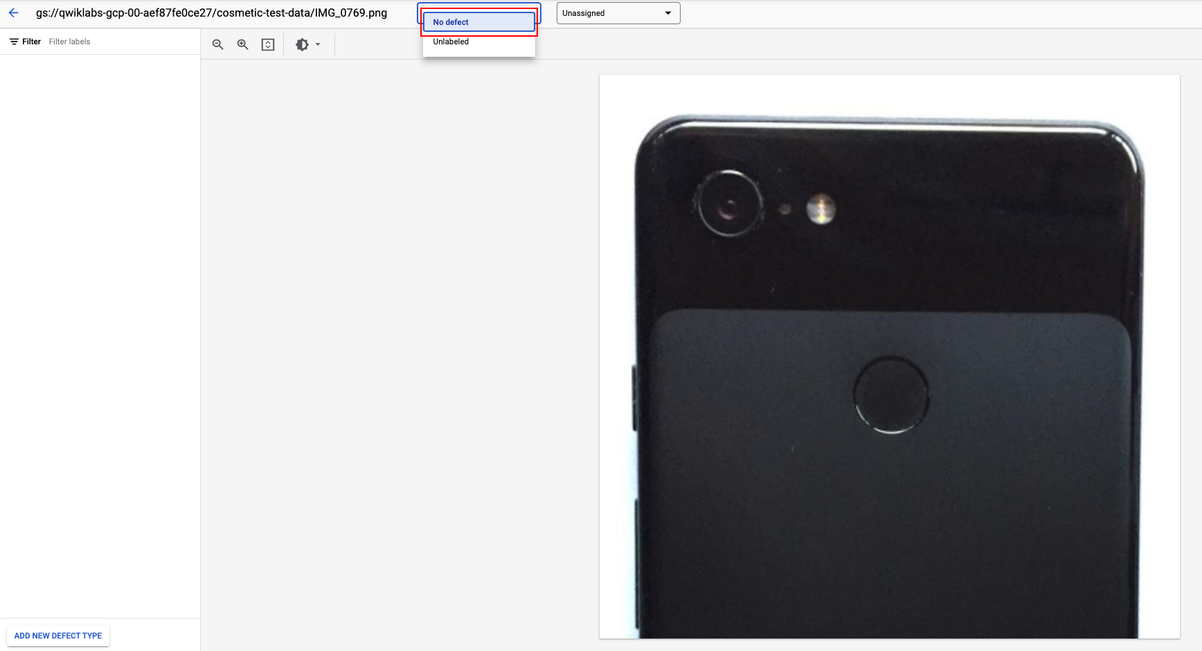
- Select an image without any defects.
Since all imported images by default do not have a label, if an image does not contain any defect instances, the image represents a non-defective or normal image, you should explicitly confirm in the UI that the image is a clean non-defective or normal image.
-
Click the drop-down at the top of the UI tab to explicitly set the image label as No defect.
-
Click Confirm to set image label as No defect.
If you were continuing the process to train a model you would now continue to annotate and label the visible defect instances for all of the remaining images in the dataset and label all of the images that are defect free with the label No defect. Since you are not proceeding to train the model you have now completed all of the tasks in the lab.
In general, the more images in the dataset with fully labelled annotations the better; however, you are not required to annotate every single image in the dataset.
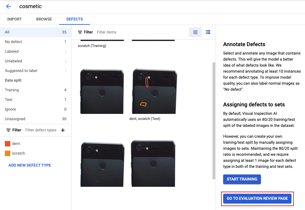
This training process takes approximately 24 hours for this sample dataset, so rather than waiting, the remainder of this lab provides an overview of the steps involved in evaluating the trained model and creating the solution artifact.
If you were training your own model you would click the button to start training at this point, but you should not do that for this lab. In the lab Deploying and Testing a Visual Inspection AI Cosmetic Anomaly Detection Solution, you learn how to deploy and use this solution artifact to analyse images.
Overview 1. Evaluating a trained Cosmetic Inspection model
This section demonstrates how to access and interpret the model evaluation user interface for a trained model.
Once the training is completed, the Go to the evaluation page button will show up on the right panel. This button opens the Model Evaluation review page.
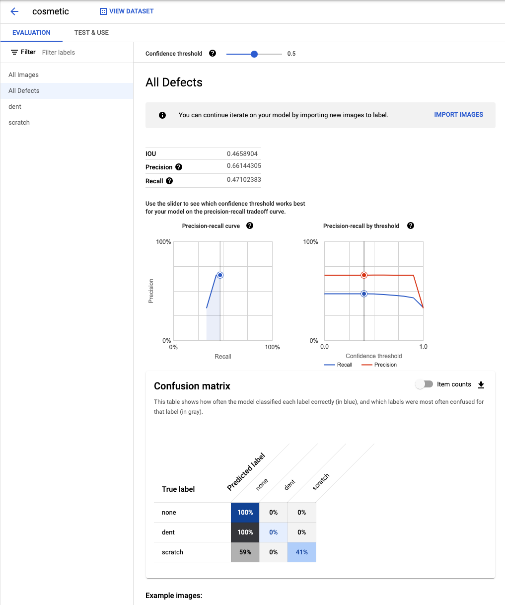
Visual Inspection AI Cosmetic Inspection reports solution-specific metrics related to the localization accuracy of the model, that is the accuracy with which the defect instance locations predicted by the model match the ground truth defect locations.
The model evaluation detailed user interface page shows the IOU, Precision and Recall model evaluation metrics for the trained Cosmetic Inspection model, where the Precision and Recall metrics here refer to the pixel-level Precision and Recall.
The page also shows the confusion matrix calculated based on the model's classification of each label. This matrix shows how often the model classified each label correctly (in blue), and which labels were most often confused for that label (in gray).
The Confidence threshold slider on the top of the Model Evaluation page can be used to see how the precision / recall evaluation metrics change with the confidence threshold.
Overview 2. Creating a trained Cosmetic Inspection solution artifact
This section provides an overview of the process of creating a trained Cosmetic Inspection solution artifact.
After evaluating the results of the trained model, a trained solution artifact can be created in a docker format, and exported to a Container Registry location.
The steps to create a trained solution artifact are as follows:
- In the Test & Use tab on the Models page for the cosmetic model, click Create Solution Artifact to create a Cosmetic Inspection solution artifact for a trained model.
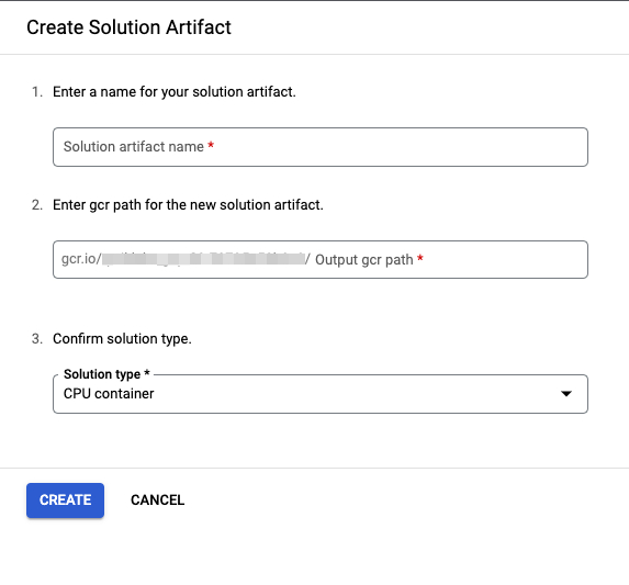
- When creating the solution artifact you must specify the Solution artifact name, Cloud Source Repository Output gcr path, and the Solution type.
- Clicking Create triggers the solution artifact container image creation process.
It usually only takes a couple of minutes to create the solution artifact.
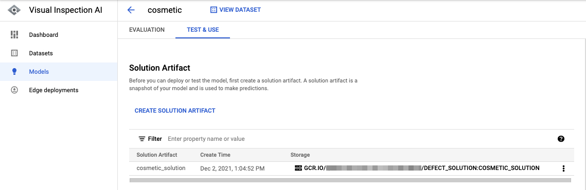
At this stage the solution artifact is now ready and can be tested in the UI. This allows you to check out the quality of the trained solution using handful of test images by running a batch prediction.
Overview 3. Performing batch predictions using a Cosmetic Inspection solution artifact
This section provides an overview of how to make batch predictions using the Cosmetic Inspection solution artifact created in the previous section.
This process can be used to check the quality of the trained solution using a handful of test images prior to deploying it to on-premise environment.
The steps to create a batch prediction job and check out the prediction results are as follows:
- On the Test & Use tab in the Models page, click Create Batch Prediction in the Test your model section to start a cloud batch prediction job using your solution container.
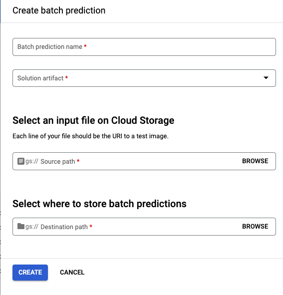
- You must provide the following details to start a batch processing task:
| Field | Value |
|---|---|
| Batch prediction name | A name for this batch prediction test |
| Solution artifact | The ID of the Solution Artifact |
| gs:// Source Path | The path to a CSV file in a Cloud Storage bucket containing the image names. |
| Destination path | The path to a Cloud Storage bucket, where the JSON output file should be stored. |
-
Click Create start the batch processing task.
-
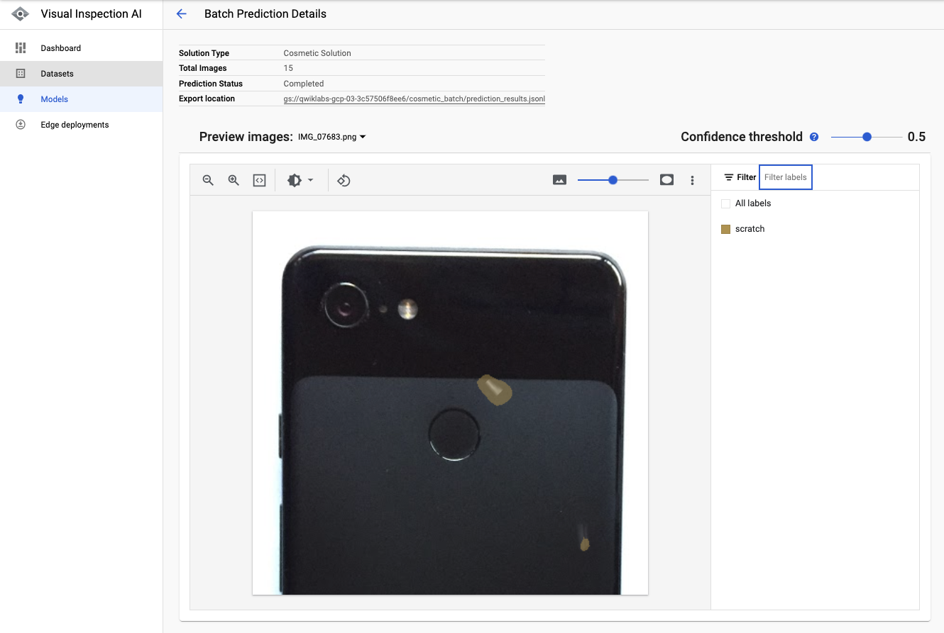
Click the Storage link of the completed batch prediction job to show the batch prediction results and details.
In the results preview page, users can change the image from the dropdown button to show the prediction results of different images, as well as play with the Confidence Threshold scrollbar to visualize the results of model prediction masks at different threshold levels.
The batch prediction data is contained in the JSON output file stored in the Cloud Storage bucket. An example of the output is shown below. You can see the data for the annotated defect that has been detected and classified as a dent as well as information about the source image.
Congratulations
Congratulations, you've successfully prepared a dataset for training a Visual Inspection AI Cosmetic Inspection model, and annotated defect instances in training images. You've also reviewed the process of training and evaluating the Cosmetic Inspection anomaly detection model, seen how to create a trained Cosmetic Inspection solution artifact and then perform batch prediction using the solution artifact.
Google Cloud training and certification
...helps you make the most of Google Cloud technologies. Our classes include technical skills and best practices to help you get up to speed quickly and continue your learning journey. We offer fundamental to advanced level training, with on-demand, live, and virtual options to suit your busy schedule. Certifications help you validate and prove your skill and expertise in Google Cloud technologies.
Manual Last Updated March 19, 2024
Lab Last September March 19, 2024
Copyright 2024 Google LLC All rights reserved. Google and the Google logo are trademarks of Google LLC. All other company and product names may be trademarks of the respective companies with which they are associated.