Overview

BigQuery is Google's fully managed, NoOps, low cost analytics database. With BigQuery you can query terabytes and terabytes of data without having any infrastructure to manage or needing a database administrator. BigQuery uses SQL and can take advantage of the pay-as-you-go model. BigQuery allows you to focus on analyzing data to find meaningful insights.

BigQuery Machine Learning is a feature in BigQuery where data analysts can create, train, evaluate, and predict with machine learning models with minimal coding.

In this lab you will use the London bicycles dataset to build a regression model in BigQuery ML to predict trip duration. Let’s say that you're a bike rental business stocking two types of bicycles -- hardy commuter bikes and fast, but fragile, road bikes. If a bicycle rental is likely to be for a long duration, we need to have road bikes in stock, but if the rental is likely to be for a short duration, we need to have commuter bikes in stock. Therefore, in order to build a system to properly stock bicycles, we need to predict the duration of bicycle rentals.

Objectives

In this lab, you learn to perform the following tasks:

• Query and explore the London bicycles dataset for feature engineering
• Create a linear regression model in BigQuery ML
• Evaluate the performance of your machine learning model
• Extract your model weights

What you'll need

• A Google Cloud Platform Project
• A Browser, such as Google Chrome or Mozilla Firefox

Set up your environment

For each lab, you get a new Google Cloud project and set of resources for a fixed time at no cost.

1. Sign in to Qwiklabs using an incognito window.

2. Note the lab's access time (for example, 1:15:00), and make sure you can finish within that time.
   There is no pause feature. You can restart if needed, but you have to start at the beginning.

3. When ready, click Start lab.

4. Note your lab credentials (Username and Password). You will use them to sign in to the Google Cloud Console.

5. Click Open Google Console.

6. Click Use another account and copy/paste credentials for this lab into the prompts.
   If you use other credentials, you'll receive errors or incur charges.

7. Accept the terms and skip the recovery resource page.

Open BigQuery Console

1. In the Google Cloud Console, on the Navigation menu , click BigQuery.
   The Welcome to BigQuery in the Cloud Console dialog opens. This dialog provides a link to the quickstart guide and lists UI updates.

2. Click Done to close the dialog.

Task 1. Explore bike data for feature engineering

The first step of solving an ML problem is to formulate it -- to identify features of our model and the label. Since the goal of our first model is to predict the duration of a rental based on our historical dataset of cycle rentals, the label is the duration of the rental.

If we believe that the duration will vary based on the station the bicycle is being rented at, the day of the week, and the time of day, those could be our features. Before we go ahead and create a model with these features, though, it’s a good idea to verify that these factors do influence the label.

Coming up with features for a machine learning model is called feature engineering. Feature engineering is often the most important part of building accurate ML models, and can be much more impactful than deciding which algorithm to use or tuning hyper-parameters. Good feature engineering requires deep understanding of the data and the domain. It is often a process of hypothesis testing; you have an idea for a feature, you check to see if it works (has mutual information with the label), and then you add it to the model. If it doesn’t work, you try again.

Impact of station

To check whether the duration of a rental varies by station, we can visualize the result of the following query in Looker Studio

1. In the query EDITOR paste the following query:

SELECT start_station_name, AVG(duration) AS duration FROM `bigquery-public-data`.london_bicycles.cycle_hire GROUP BY start_station_name

2. Click on RUN.
3. Click on OPEN IN > Looker Studio in the BigQuery Cloud Console.
4. When prompted, select the GET STARTED button.
5. Click on the Chart, present on the canvas.
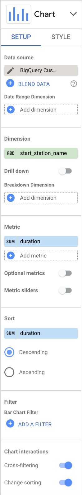
6. In the SETUP tab on the right-hand side menu, configure the settings as follows:

• Dimension: start_station_name
• Metric: duration
• Sort: by duration in Descending order.
• Chart Interaction: Enable both Cross filtering and Change sorting.

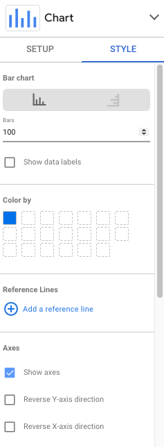
7. In the STYLE tab on the right-hand side menu, configure the settings as follows:

• Bar chart: Vertical

• Bars: 100

• Axes: Show axes

  

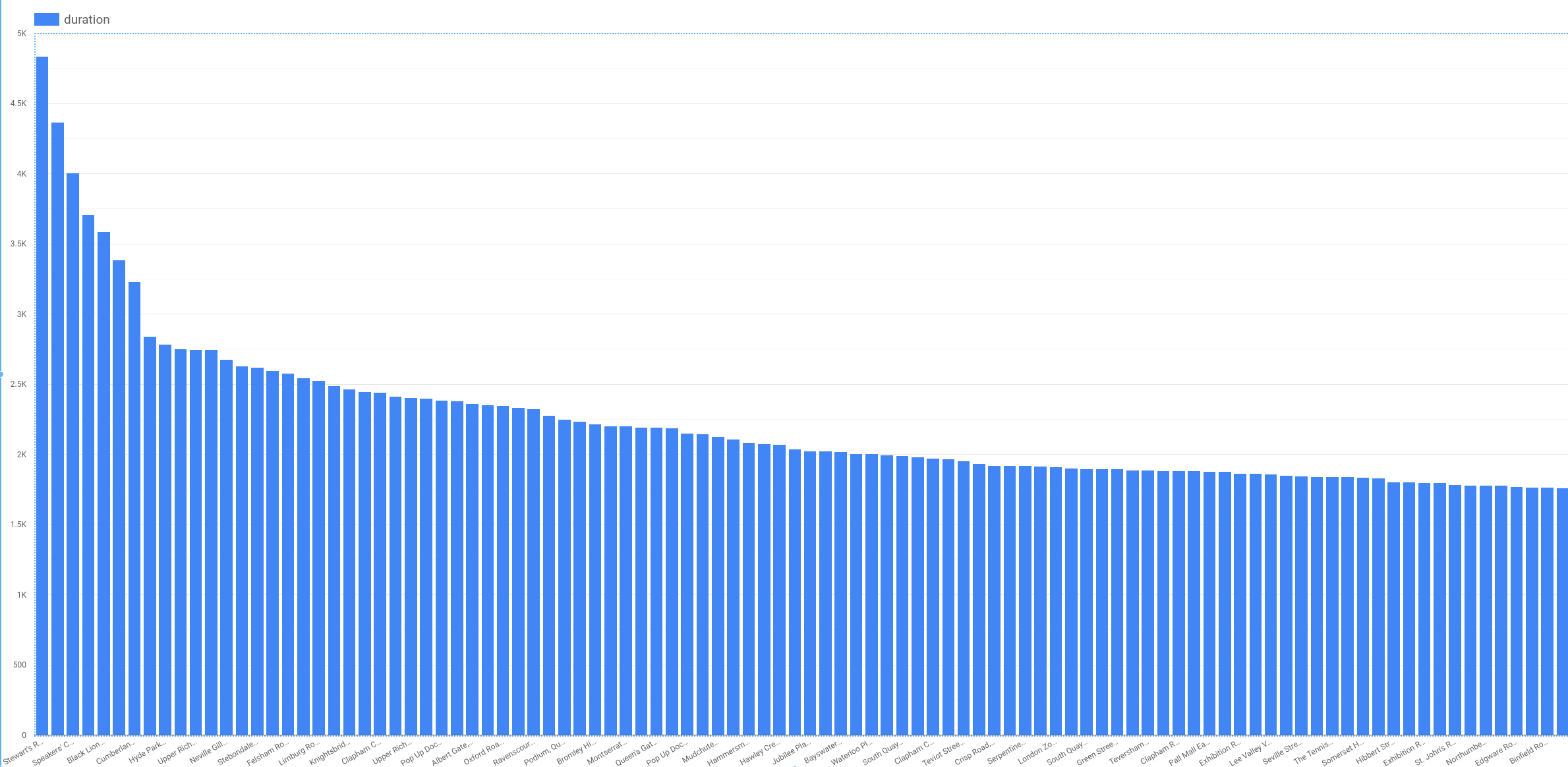
Your plot should resemble this:

It is clear that a handful of stations are associated with long-duration rentals (over 3000 seconds), but that the majority of stations have durations that lie in a relatively narrow range. Had all the stations in London been associated with durations within a narrow range, the station at which the rental commenced would not have been a good feature. But in this problem, as the graph demonstrates, the start_station_name does matter.

Note: We cannot use end_station_name as a feature because at the time the bicycle is being rented, we won’t know where the bicycle is going to be returned to.

Because we are creating a machine learning model to predict events in the future, we need to be mindful of not using any columns that will not be known at the time the prediction is made. This time/causality criterion imposes constraints on what features we can use.

Impact of day of week and hour of day

For the next candidate features, the process is similar. We can check whether dayofweek (or, similarly, hourofday) matter.

1. In the query editor window paste the following query:

SELECT EXTRACT(dayofweek FROM start_date) AS dayofweek, AVG(duration) AS duration FROM `bigquery-public-data`.london_bicycles.cycle_hire GROUP BY dayofweek

2. Click on OPEN IN > Looker Studio in the BigQuery Cloud Console.

Note: If you see a System Error message, you need to make some changes to visualize the data in Looker Studio outlined in steps 3 to 11.

3. Click the table which contains the duration and dayofweek data.

4. In Setup > Metric, hover over dayofweek and click edit pencil icon.

5. From the Display format dropdown, click Week Number, then choose Custom date format.

6. Change the custom date to 'Day' w and then click Apply. In the graph, the field dayofweek now displays Day1 to Day 7.

7. Click the chart which shows System Error.

8. In Setup > Dimension, click Duration and change to dayofweek.

9. In Setup > Dimension, hover over dayofweek and click edit pencil icon.

10. From the Display format dropdown, select Custom date format and change the custom date to 'Day' w. Then click Apply.

11. In Setup > Metric, click dayofweek and change to duration.

For day of week your visualization should resemble:

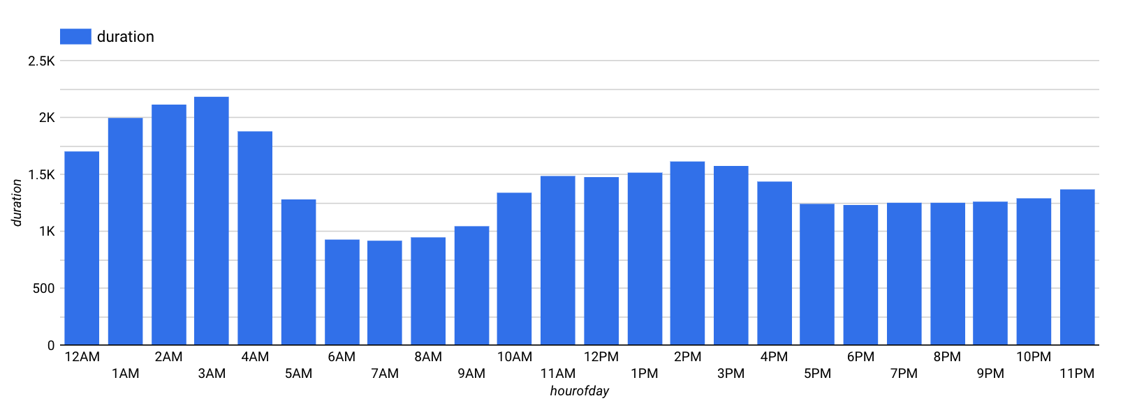
For hour of day your visualization should look like the following:

Note: As in the previous steps, you may need to modify the properties in Looker Studio to see the desired output.

It is clear that the duration varies depending both on the day of the week, and on the hour of the day. It appears that durations are longer on weekends (days 1 and 7) than on weekdays. Similarly, durations are longer early in the morning and in the mid-afternoon. Hence, both dayofweek and hourofday are good features.

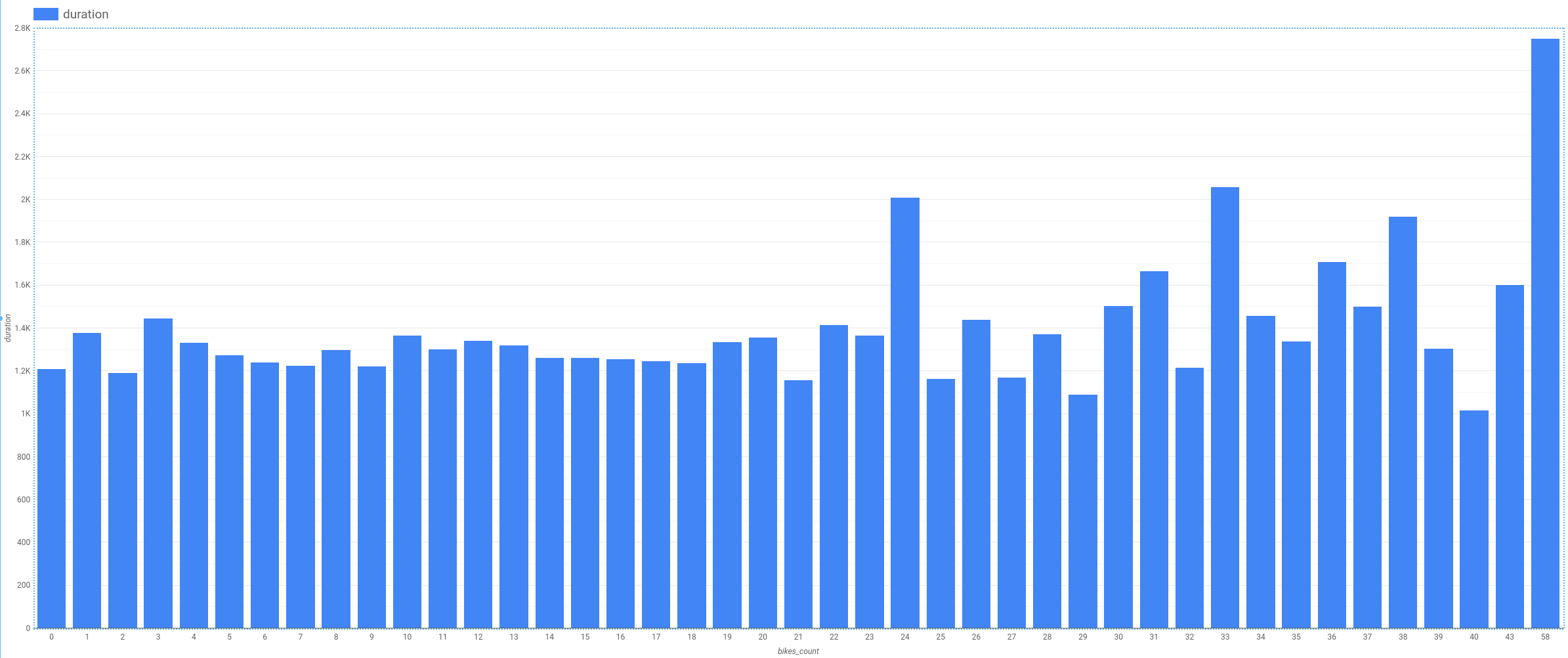
Impact of number of bicycles

Another potential feature is the number of bikes in the station. Perhaps, we hypothesize, people keep bicycles longer if there are fewer bicycles on rent at the station they rented from.

1. In the query editor window paste the following query:

SELECT bikes_count, AVG(duration) AS duration FROM `bigquery-public-data`.london_bicycles.cycle_hire JOIN `bigquery-public-data`.london_bicycles.cycle_stations ON cycle_hire.start_station_name = cycle_stations.name GROUP BY bikes_count

2. Visualize your data in Looker Studio.

We notice that the relationship is noisy with no visible trend (compare against hour-of-day, for example). This indicates that the number of bicycles is not a good feature.

Task 2. Create a training dataset

Based on the exploration of the bicycles dataset and the relationship of various columns to the label column, we can prepare the training dataset by pulling out the selected features and the label:

SELECT duration, start_station_name, CAST(EXTRACT(dayofweek FROM start_date) AS STRING) AS dayofweek, CAST(EXTRACT(hour FROM start_date) AS STRING) AS hourofday FROM `bigquery-public-data`.london_bicycles.cycle_hire

Feature columns have to be either numeric (INT64, FLOAT64, etc.) or categorical (STRING). If the feature is numeric but needs to be treated as categorical, we need to cast it as a string -- this explains why we casted the dayofweek and hourofday columns which are integers (in the ranges 1-7 and 0-23, respectively) into strings.

If preparing the data involves computationally expensive transformations or joins, it might be a good idea to save the prepared training data as a table so as to not repeat that work during experimentation. If the transformations are trivial but the query itself is long-winded, it might be convenient to avoid repetitiveness by saving it as a view.

In this case, the query is simple and short, and so, for clarity, we won't be saving it.

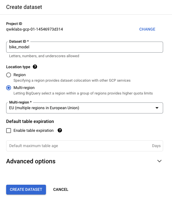
1. Create a dataset in BigQuery called bike_model to store your model. Set the Location type to Multi-region and select EU (multiple regions in European Union) region since the data we are training on is in the EU. Click Create dataset.

To train the ML model and save it into the dataset bike_model, we need to call CREATE MODEL, which works similarly to CREATE TABLE. Since the label we're trying to predict is numeric this is a regression problem, which is why the most appropriate option is to choose linear_reg as the model type under OPTIONS.

2. Enter the following query into the query editor:

CREATE OR REPLACE MODEL bike_model.model OPTIONS (input_label_cols=['duration'], model_type='linear_reg') AS SELECT duration, start_station_name, CAST(EXTRACT(dayofweek FROM start_date) AS STRING) AS dayofweek, CAST(EXTRACT(hour FROM start_date) AS STRING) AS hourofday FROM `bigquery-public-data`.london_bicycles.cycle_hire WHERE `duration` IS NOT NULL

Note, the model takes 2-3 minutes to train.

3. To see some metrics related to model training, enter the following query into the BigQuery editor window:

SELECT * FROM ML.EVALUATE(MODEL `bike_model.model`)

The mean absolute error is 1025 seconds or about 17 minutes. This means that we should expect to be able to predict the duration of bicycle rentals with an average error of about 17 minutes.

Click Check my progress to verify the objective. Create a training dataset

Task 3. Improving the model through feature engineering

Combine days of week

There are other ways that we could have chosen to represent the features that we have. For example, recall that when we explored the relationship between dayofweek and the duration of rentals, we found that durations were longer on weekends than on weekdays. Therefore, instead of treating the raw value of dayofweek as a feature, we can employ this insight by fusing several dayofweek values into the weekday category

1. Build a BigQuery ML model with the combined days of week feature using the following query:

CREATE OR REPLACE MODEL bike_model.model_weekday OPTIONS (input_label_cols=['duration'], model_type='linear_reg') AS SELECT duration, start_station_name, IF (EXTRACT(dayofweek FROM start_date) BETWEEN 2 AND 6, 'weekday', 'weekend') AS dayofweek, CAST(EXTRACT(hour FROM start_date) AS STRING) AS hourofday FROM `bigquery-public-data`.london_bicycles.cycle_hire WHERE `duration` IS NOT NULL

2. To see the metrics for this model, enter the following query into the BigQuery editor window:

SELECT * FROM ML.EVALUATE(MODEL `bike_model.model_weekday`)

This model results in a mean absolute error of 966 seconds which is less than the 1025 seconds for the original model. Improvement!

Bucketize hour of day

Based on the relationship between hourofday and the duration, we can experiment with bucketizing the variable into 4 bins; (-inf,5), [5,10), [10,17), and [17,inf).

1. Build a BigQuery ML model with the bucketized hour of day, and combined days of week features using the query below:

CREATE OR REPLACE MODEL bike_model.model_bucketized OPTIONS (input_label_cols=['duration'], model_type='linear_reg') AS SELECT duration, start_station_name, IF (EXTRACT(dayofweek FROM start_date) BETWEEN 2 AND 6, 'weekday', 'weekend') AS dayofweek, ML.BUCKETIZE(EXTRACT(hour FROM start_date), [5, 10, 17]) AS hourofday FROM `bigquery-public-data`.london_bicycles.cycle_hire WHERE `duration` IS NOT NULL

2. To see the metrics for this model, enter the following query into the BigQuery editor window:

SELECT * FROM ML.EVALUATE(MODEL `bike_model.model_bucketized`)

This model results in a mean absolute error of 904 seconds which is less than the 966 seconds for the weekday-weekend model. Further improvement!

Click Check my progress to verify the objective. Improving the model through feature engineering

Task 4. Make predictions

Our best model contains several data transformations. Wouldn’t it be nice if BigQuery could remember the sets of transformations we did at the time of training and automatically apply them at the time of prediction? It can, using the TRANSFORM clause!

In this case, the resulting model requires just the start_station_name and start_date to predict the duration. The transformations are saved and carried out on the provided raw data to create input features for the model. The main advantage of placing all preprocessing functions inside the TRANSFORM clause is that clients of the model do not have to know what kind of preprocessing has been carried out.

1. Build a BigQuery ML model with the TRANSFORM clause that incorporates the bucketized hour of day, and combined days of week features using the query below:

CREATE OR REPLACE MODEL bike_model.model_bucketized TRANSFORM(* EXCEPT(start_date), IF (EXTRACT(dayofweek FROM start_date) BETWEEN 2 AND 6, 'weekday', 'weekend') AS dayofweek, ML.BUCKETIZE(EXTRACT(HOUR FROM start_date), [5, 10, 17]) AS hourofday ) OPTIONS (input_label_cols=['duration'], model_type='linear_reg') AS SELECT duration, start_station_name, start_date FROM `bigquery-public-data`.london_bicycles.cycle_hire WHERE `duration` IS NOT NULL

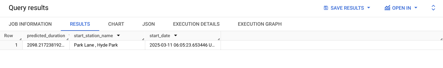
2. With the TRANSFORM clause in place, enter this query to predict the duration of a rental from Park Lane right now (your result will vary):

SELECT * FROM ML.PREDICT(MODEL bike_model.model_bucketized, ( SELECT 'Park Lane , Hyde Park' AS start_station_name, CURRENT_TIMESTAMP() AS start_date) )

3. To make batch predictions on a sample of 100 rows in the training set use the query:

SELECT * FROM ML.PREDICT(MODEL bike_model.model_bucketized, ( SELECT start_station_name, start_date FROM `bigquery-public-data`.london_bicycles.cycle_hire LIMIT 100) )

Click Check my progress to verify the objective. Make predictions

Task 5. Examine model weights

A linear regression model predicts the output as a weighted sum of its inputs. Often times, the weights of the model need to be utilized in a production environment.

• Examine (or export) the weights of your model using the query below:

  SELECT * FROM ML.WEIGHTS(MODEL bike_model.model_bucketized)

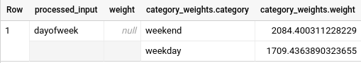
  Note, numeric features get a single weight, while categorical features get a weight for each possible value. For example, the dayofweek feature has the following weights:

  

  This means that if the day is a weekday, the contribution of this feature to the overall predicted duration is 1709 seconds (the weights that provide the optimal performance are not unique, so you might get a different value).

  Click Check my progress to verify the objective. Examine model weights

End your lab

When you have completed your lab, click End Lab. Qwiklabs removes the resources you’ve used and cleans the account for you.

You will be given an opportunity to rate the lab experience. Select the applicable number of stars, type a comment, and then click Submit.

The number of stars indicates the following:

• 1 star = Very dissatisfied
• 2 stars = Dissatisfied
• 3 stars = Neutral
• 4 stars = Satisfied
• 5 stars = Very satisfied

You can close the dialog box if you don't want to provide feedback.

For feedback, suggestions, or corrections, please use the Support tab.

Copyright 2022 Google LLC All rights reserved. Google and the Google logo are trademarks of Google LLC. All other company and product names may be trademarks of the respective companies with which they are associated.