GSP852

Overview

BigQuery is Google's fully managed, NoOps, low cost analytics database. With BigQuery you can query terabytes and terabytes of data without having any infrastructure to manage, or needing a database administrator.

BigQuery Machine Learning (BQML) is a feature in BigQuery where data analysts can create, train, evaluate, and predict with machine learning models with minimal coding. Watch this BigQuery ML video to learn more.

In this lab, you will learn how to build a time series model to forecast the demand of multiple products using BigQuery ML. Using the NYC Citi Bike Trips public dataset, learn how to use historical data to forecast demand in the next 30 days. Imagine the bikes are retail items for sale, and the bike stations are stores.

Watch this video to understand some example use cases for demand forecasting.

What you'll learn

In this lab, you learn to perform the following tasks:

• Use BigQuery to find public datasets.
• Query and explore the public NYC Citi Bike Trips dataset.
• Create a training and evaluation dataset to be used for batch prediction.
• Create a forecasting (time series) model in BQML.
• Evaluate the performance of your machine learning model.

Setup and requirements

Before you click the Start Lab button

Read these instructions. Labs are timed and you cannot pause them. The timer, which starts when you click Start Lab, shows how long Google Cloud resources are made available to you.

This hands-on lab lets you do the lab activities in a real cloud environment, not in a simulation or demo environment. It does so by giving you new, temporary credentials you use to sign in and access Google Cloud for the duration of the lab.

To complete this lab, you need:

• Access to a standard internet browser (Chrome browser recommended).

Note: Use an Incognito (recommended) or private browser window to run this lab. This prevents conflicts between your personal account and the student account, which may cause extra charges incurred to your personal account.

• Time to complete the lab—remember, once you start, you cannot pause a lab.

Note: Use only the student account for this lab. If you use a different Google Cloud account, you may incur charges to that account.

How to start your lab and sign in to the Google Cloud console

1. Click the Start Lab button. If you need to pay for the lab, a dialog opens for you to select your payment method. On the left is the Lab Details pane with the following:

   • The Open Google Cloud console button
   • Time remaining
   • The temporary credentials that you must use for this lab
   • Other information, if needed, to step through this lab

2. Click Open Google Cloud console (or right-click and select Open Link in Incognito Window if you are running the Chrome browser).

   The lab spins up resources, and then opens another tab that shows the Sign in page.

   Tip: Arrange the tabs in separate windows, side-by-side.

   Note: If you see the Choose an account dialog, click Use Another Account.

3. If necessary, copy the Username below and paste it into the Sign in dialog.

   {{{user_0.username | "Username"}}}

   You can also find the Username in the Lab Details pane.

4. Click Next.

5. Copy the Password below and paste it into the Welcome dialog.

   {{{user_0.password | "Password"}}}

   You can also find the Password in the Lab Details pane.

6. Click Next.

   Important: You must use the credentials the lab provides you. Do not use your Google Cloud account credentials. Note: Using your own Google Cloud account for this lab may incur extra charges.

7. Click through the subsequent pages:

   • Accept the terms and conditions.
   • Do not add recovery options or two-factor authentication (because this is a temporary account).
   • Do not sign up for free trials.

After a few moments, the Google Cloud console opens in this tab.

Note: To access Google Cloud products and services, click the Navigation menu or type the service or product name in the Search field.

Open the BigQuery console

1. In the Google Cloud Console, select Navigation menu > BigQuery.

The Welcome to BigQuery in the Cloud Console message box opens. This message box provides a link to the quickstart guide and the release notes.

2. Click Done.

The BigQuery console opens.

Task 1. Explore the NYC Citi Bike Trips dataset

You will use the public dataset for NYC Bike Trips. This dataset can be accessed in Marketplace within the Google Cloud console. BigQuery makes it easy to access public datasets directly from the Explorer interface.

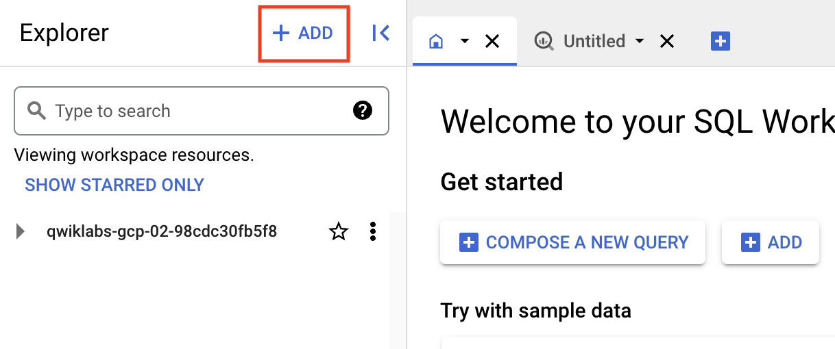
1. In the Explorer pane, click + Add data.

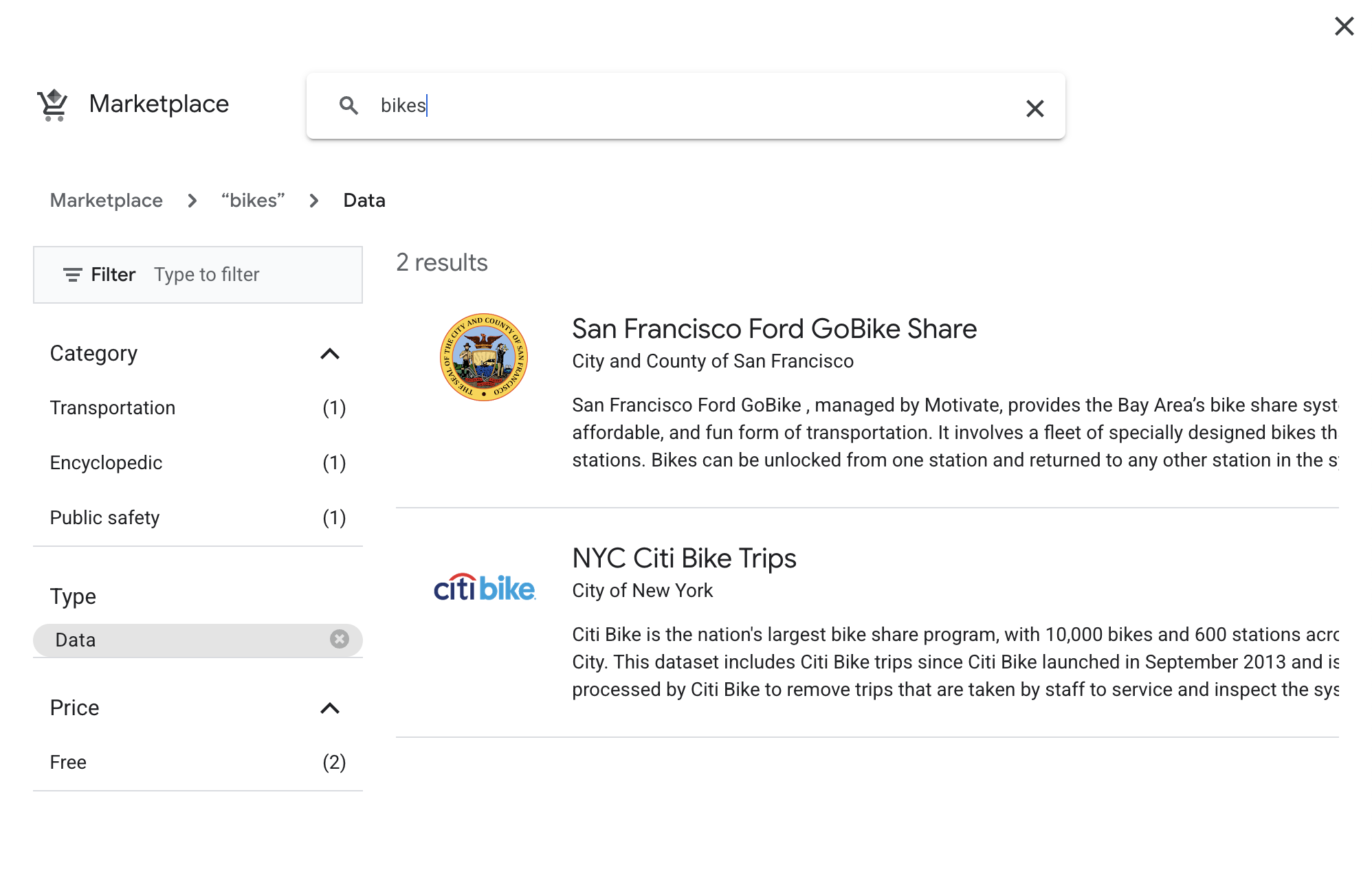
2. Under Additional Sources, select Public Datasets.

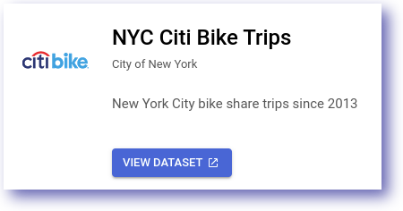
3. Search for "bikes" and click on the NYC Citi Bike Trips tile.

4. Click the View dataset button to open the dataset in BigQuery:

Question: Could you name some New York locations where you can hire bikes?

Next you'll make a query to answer that question.

5. Click on the Editor tab, then add the following SQL code into the query Editor:

SELECT bikeid, starttime, start_station_name, end_station_name, FROM `bigquery-public-data.new_york_citibike.citibike_trips` WHERE starttime is not null LIMIT 5

6. Then click Run.
7. You should see a table structure similar to below:

Row	bikeid	starttime	start_station_name	end_station_name
1	18447	2013-09-16T19:22:43	9 Ave & W 22 St	W 27 St & 7 Ave
2	22598	2015-12-30T13:02:38	E 10 St & 5 Ave	W 11 St & 6 Ave
3	28833	2017-09-02T16:27:37	Washington Pl & Broadway	Lexington Ave & E 29 St
4	21338	2017-11-15T06:57:09	Hudson St & Reade St	Centre St & Chambers St
5	19888	2013-11-07T15:12:07	W 42 St & 8 Ave	W 56 St & 6 Ave

This is a list of station locations in New York City where you can hire a bike. You now know how to query the Citi Bike trips dataset.

Test completed task

BigQuery is great for answering questions through data. Learning the query syntax will assist in providing insight through data.

Thinking about the query that was just run...

Try another type of query. In some instances, it may be useful to filter a dataset to present a more granular view.

In the following example, use BigQuery to implement a date range.

1. Replace the previous query with the following:

SELECT EXTRACT (DATE FROM TIMESTAMP(starttime)) AS start_date, start_station_id, COUNT(*) as total_trips FROM `bigquery-public-data.new_york_citibike.citibike_trips` WHERE starttime BETWEEN DATE('2016-01-01') AND DATE('2017-01-01') GROUP BY start_station_id, start_date LIMIT 5 Note: In the above query a new keyword was introduced:

GROUP BY: Combine non-distinct values

2. Now click Run.

You should receive a result similar to the following:

Row	start_date	start_station_id	total_trips
1	2016-01-27	3119	15
2	2016-04-07	3140	83
3	2016-08-15	254	109
4	2016-05-10	116	217
5	2016-07-07	268	151

Note: The data has been transformed from its original state. Being able to transform data is a useful skill when consuming datasets you do not own.

start_date: TIMESTAMP to a DATE

total_trip: COUNT of rows

You now know how to filter query results by date range.

Test completed task

Building queries involves learning commands to manipulate the data. Based on the last query you can now group the trips by date and station name.

Click Check my progress to verify the objective. Explore the NYC Citi Bike Trips dataset

Task 2. Cleaned training data

From the last query run, you now have one row per date, per start_station, and the number of trips for that day. This data can be stored as a table or view.

In the next section you will create the following structure for your training data:

Type	Name
Dataset	bqmlforecast
Table	training_data

Create a dataset

1. In the Explorer pane, click on the three dots next to your project that starts with "qwiklabs" to see the Create Dataset option.
2. Select Create Dataset.
3. Enter the dataset name as bqmlforecast.
4. Click Advanced options, and then check the box for Enable table expiration and enter 1 day for Default maximum table age
5. Select the Create dataset button.

You now have a dataset in which to host your data.

Create the table

Unfortunately you do not currently have any data created. Correct that by running a query and saving the results to a table.

1. Click the + (SQL query) button.
2. Run the following query to generate some data:

SELECT DATE(starttime) AS trip_date, start_station_id, COUNT(*) AS num_trips FROM `bigquery-public-data.new_york_citibike.citibike_trips` WHERE starttime BETWEEN DATE('2014-01-01') AND ('2016-01-01') AND start_station_id IN (521,435,497,293,519) GROUP BY start_station_id, trip_date Note: The IN clause chooses just 5 of the stations to include in the model to reduce the size of the training data. Training a full model requires more time than is available for this lab. You can now use this query as the basis for training our model.

3. Select Save results.
4. In the dropdown menu, select BigQuery table.
5. For Dataset select bqmlforecast.
6. Add a Table name training_data .
7. Click Save.

Click Check my progress to verify the objective. Cleaned training data

Task 3. Training a model

The next query will use the training data to create a ML model. The model produced will enable you to perform demand forecasting.

Note: In the query below you are using the ARIMA algorithm for time series forecasting. Other algorithms are available and can be found in the BigQuery ML documentation.

1. Enter the following query into the Editor:

CREATE OR REPLACE MODEL bqmlforecast.bike_model OPTIONS( MODEL_TYPE='ARIMA', TIME_SERIES_TIMESTAMP_COL='trip_date', TIME_SERIES_DATA_COL='num_trips', TIME_SERIES_ID_COL='start_station_id', HOLIDAY_REGION='US' ) AS SELECT trip_date, start_station_id, num_trips FROM bqmlforecast.training_data

2. Click Run to initiate training.
3. BigQuery will now begin training the model. It will take approximately 2 minutes for the training to complete. While you're waiting, continue reading about what's happening right now.

When you train a time series model with BigQuery ML, multiple models/components are used in the model creation pipeline. ARIMA is one of the core algorithms available in BigQuery ML.

The components used are listed in roughly the order of the steps that are run:

• Pre-processing: Automatic cleaning adjustments to the input time series, including missing values, duplicated timestamps, spike anomalies, and accounting for abrupt level changes in the time series history.
• Holiday effects: Time series modeling in BigQuery ML can also account for holiday effects. By default, holiday effects modeling is disabled. But since this data is from the United States, and the data includes a minimum one year of daily data, you can also specify an optional HOLIDAY_REGION. With holiday effects enabled, spike and dip anomalies that appear during holidays will no longer be treated as anomalies. A full list of the holiday regions can be found in the HOLIDAY_REGION documentation.
• Seasonal and trend decomposition using the Seasonal and Trend decomposition using LOgical regrESSion (Loess STL) algorithm. Seasonality extrapolation using the double exponential smoothing (ETS) algorithm.
• Trend modeling using the ARIMA model and the auto. ARIMA algorithm for automatic hyper-parameter tuning. In auto.ARIMA, dozens of candidate models are trained and evaluated in parallel, which include p,d,q and drift. The best model comes with the lowest Akaike information criterion (AIC).

You can train a time series model to forecast a single item, or forecast multiple items at the same time (which is really convenient if you have thousands or millions of items to forecast).

To forecast multiple items at the same time, different pipelines are run in parallel.

In this example, since you are training the model on multiple stations in a single model creation statement, you will need to specify the parameter TIME_SERIES_ID_COL as start_station .

If you are only forecasting a single item, then you would not need to specify TIME_SERIES_ID_COL .

When you see a green check mark the model has successfully completed, and you can use it to perform a forecast!

If you are still waiting for your model to train, you can start watching this YouTube video that discusses building and deploying a demand forecasting solution just like this lab but with a different data set. Just remember to come back to your lab - remember, this lab is only available for a set amount of time!

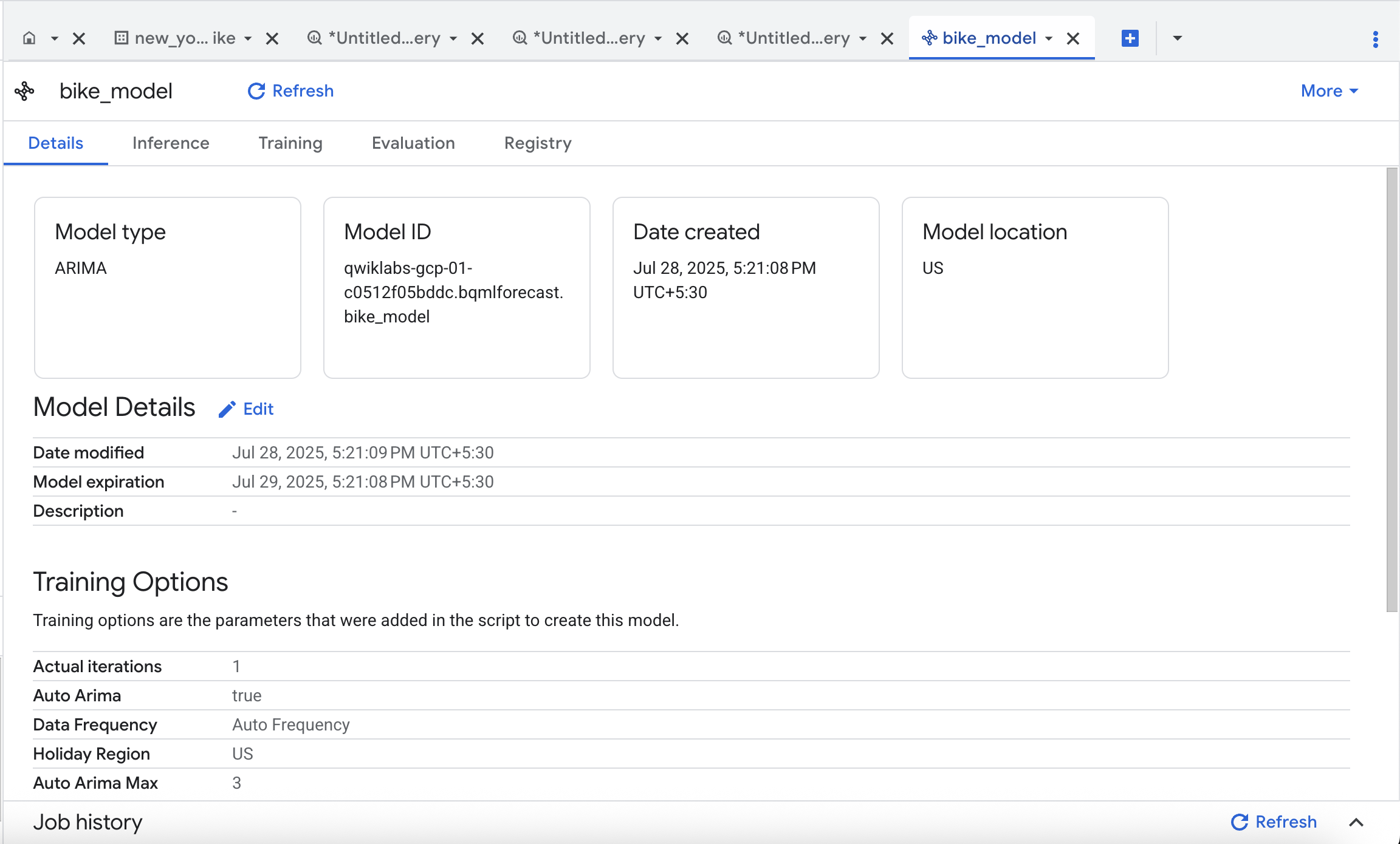
4. When the training job is finished, click on Go to model in the results tab.

Thinking about the query that was just run...

Click Check my progress to verify the objective. Training a Model

Task 4. Evaluate the time series model

Watch How time series models work in BigQuery ML to understand how time series models work in BigQuery ML.

The model produced can be queried. Based on the prior query you now have a new model available. You can use the ML.EVALUATE function (documentation) to see the evaluation metrics of all the created models (one per item):

• Query the time series model created earlier:

SELECT * FROM ML.EVALUATE(MODEL bqmlforecast.bike_model)

Running the above query should provide results similar to the image below:

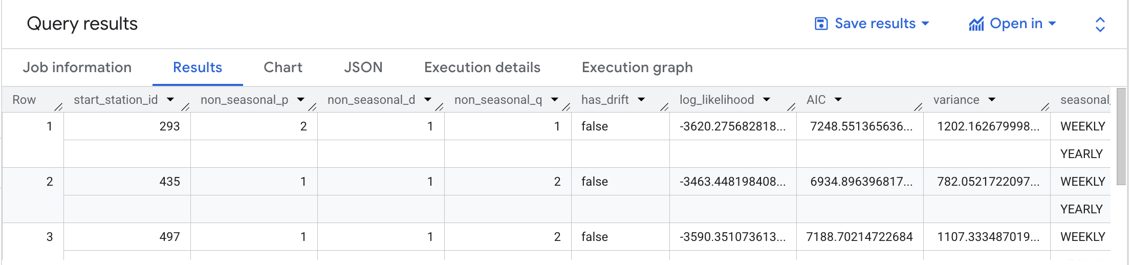
There are five models trained, one for each of the stations in the training data.

• The first four columns (non_seasonal_{p,d,q} and has_drift) define the ARIMA model.
• The next three metrics (log_likelihood, AIC, and variance) are relevant to the ARIMA model fitting process.

The fitting process determines the best ARIMA model by using the auto.ARIMA algorithm, one for each time series. Of these metrics, AIC is typically the go-to metric to evaluate how well a time series model fits the data while penalizing overly complex models.

Finally, the seasonal_periods detected for the five stations are defined as WEEKLY and YEARLY.

Try another question:

Click Check my progress to verify the objective. Evaluate the time series model

Task 5. Make predictions using the model

Make predictions using ML.FORECAST (syntax documentation), which forecasts the next n values, as set in horizon.

You can also change the confidence_level, the percentage that the forecasted values fall within the prediction interval.

The code below shows a forecast horizon of "30", which means to make predictions on the next 30 days, since the training data was daily.

1. Run the following to make a prediction for the next 30 days using the trained model:

DECLARE HORIZON STRING DEFAULT "30"; #number of values to forecast DECLARE CONFIDENCE_LEVEL STRING DEFAULT "0.90"; EXECUTE IMMEDIATE format(""" SELECT * FROM ML.FORECAST(MODEL bqmlforecast.bike_model, STRUCT(%s AS horizon, %s AS confidence_level) ) """, HORIZON, CONFIDENCE_LEVEL)

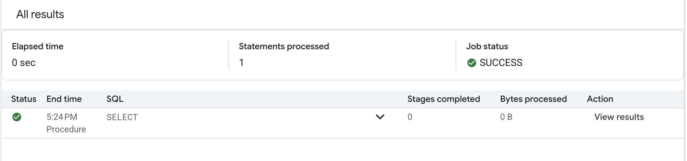
2. In the results pane, click View results under Action.

This will show results similar to below:

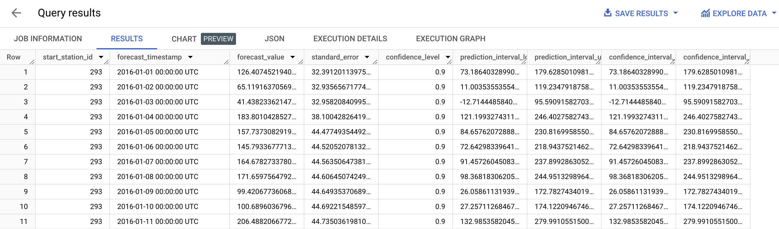
Note: Since the horizon was set to 30, the result contains 30 days of forecasts for each start_station_id. Each forecasted value also shows the upper and lower bound of the prediction_interval, given the confidence_level.

As you may notice that the SQL script uses DECLARE and EXECUTE IMMEDIATE to help parameterize the inputs for horizon and confidence_level.

As these HORIZON and CONFIDENCE_LEVEL variables make it easier to adjust the values later, this can improve code readability and maintainability.

Learn more about how this syntax works from the Query syntax reference.

Thinking about the query that was just run...

In addition to the above, BigQuery ML also supports scheduled queries. To learn more about scheduled queries, watch Scheduling and automating model retaining with scheduled queries.

Click Check my progress to verify the objective. Make Predictions using the model

Task 6. Other datasets to explore

• You can use the link below to bring in the bigquery-public-data to your own project if you want to explore modeling on other datasets, like forecasting fares for Chicago taxi trips:

  • public-data::chicago_taxi_trips.taxi_trips

Congratulations!

You've successfully built a ML model in BigQuery to perform demand forecasting.

Next steps / Learn more

To learn more about this subject from developer advocate Polong Lin see:

• YouTube - How to build and deploy a demand forecasting solution with BigQuery ML (12 minutes)
• Google Cloud blog - How to build demand forecasting models with BigQuery ML

Here is another example of how to use demand forecasting:

• Towards Data Science blog - How to do time series forecasting in BigQuery

Learn more about the tools used in this lab:

• BigQuery documentation
• For Machine Learning, see AI Platform documentation.

Google Cloud training and certification

...helps you make the most of Google Cloud technologies. Our classes include technical skills and best practices to help you get up to speed quickly and continue your learning journey. We offer fundamental to advanced level training, with on-demand, live, and virtual options to suit your busy schedule. Certifications help you validate and prove your skill and expertise in Google Cloud technologies.

Manual Last Updated August 21, 2025

Lab Last Tested August 21, 2025

Copyright 2025 Google LLC. All rights reserved. Google and the Google logo are trademarks of Google LLC. All other company and product names may be trademarks of the respective companies with which they are associated.